Tube deflection (scalar QoI)
Introduction
In this tutorial, we will show how the mUQSA platform can be used for Uncertainty Quantification and Sensitivity Analysis for an example tube deflection model.
The presented model measures the vertical deflection of a circular metal tube, suspended at each end, in a certain point along its length where a force is given.
The model is parametrised with the following parameters:
- F: the strength,
- L: the length of the tube,
- a: position of the force,
- D: external diameter of the tube,
- d: internal diameter of the tube,
- E: Young modulus.
More details about this model are available at this link.
Due to its simplicity, the model will allow you to get familiar with basic UQ & SA concepts without any background in the field.
It is worth to note that the tutorial has been based on its equivalent created for the pure EasyVVUQ library by Vytautas Jancauskas. You can see the original version here.
Note
In this tutorial we will present the usage of mUQSA deployed in our test environment, thus you may need to adapt a few settings (e.g. path to the executable) when you will use mUQSA deployed in a different location.
Application preparation
In order to employ mUQSA for the UQ&SA of a specific application, you need to take care of the preparation of this app, so it can be executed on a cluster. The basic option is to install it on a cluster and then reference to it from mUQSA, while the other is to use Apptainer/Singularity image that already contains the application. In this tutorial, we will focus on the former option.
Installing application on a cluster
Since the tube deflection application is only a python file, it can be installed on a cluster quite easily.
Log-in into the cluster
ssh test@test.clusterGet the application by cloning it from the git repository
git clone https://gitlab.pcss.pl/muqsa/muqsa-examples.git
The application called beam is available in the ./muqsa-examples/tube_deflection.
Opening mUQSA (QCG-Portal)
In order to set up the execution of UQ/SA scenario with mUQSA, please log into QCG-Portal, which offers the mUQSA service (please note that you can also be redirected automatically to QCG-Portal from other services where you are already logged in):

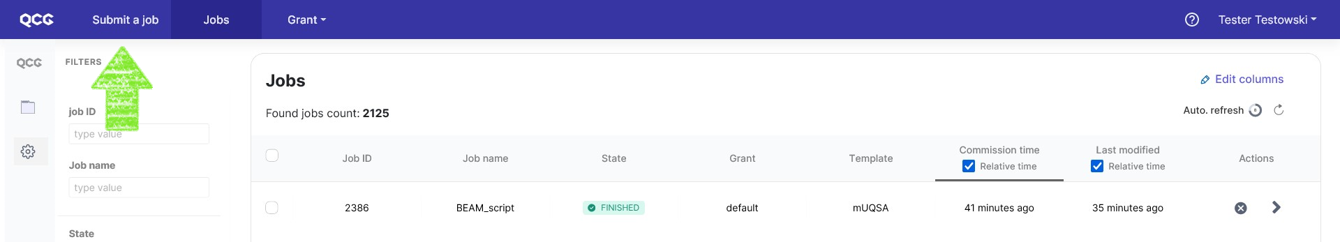
Once logged in, the main view of the portal is displayed. We can see here a list of our tasks submitted with QCG-Portal to the execution on a cluster. Click on the Submit new button to define a new task:
A template selection view is now displayed. Since we are interested in mUQSA, please look for the mUQSA template and click Submit a job on it to initiate definition of a mUQSA scenario.

Now a welcome page of the mUQSA platform is presented. It is convenient to switch to its full-screen version by clicking the appropriate icon in the top-right corner.

Scenario setup
Now we are ready to move to the essence of our UQ/SA scenario preparation.
mUQSA welcome page allows you to load an already prepared scenario definition from a file, to which it was previously saved, or to create a one from scratch. We will follow the second option by clicking Assign new task.

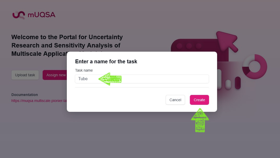
Step 0. Name
Before we start configuring the scenario, we need to give it a name. Only alphanumeric characters and underscore are allowed. For simplicity, we will call our scenario “Tube”.
Once accepted, you will be redirected to the 6-step mUQSA wizard, which will help us to set up all aspects of the scenario configuration.
Step 1. Parameters
The parameters section allows us to define a sampling space for the input parameters to our model. Depending on the variability of an input parameter, we may need to define its name, type, probability distribution along with its settings, default value and bounds.
Info
Proper selection of parameter distribution improves convergence rates of UQ/SA algorithms. If you are not sure what distribution your input parameter comes from, then the uniform distribution may be the only reliable choice.
In the case of Tube Deflection model, we consider the following list of parameters:
| Parameter Name | Type | Distribution | Default Value | Lower Bound | Upper Bound |
|---|---|---|---|---|---|
| F | float | Normal(1, 0.1) | 1.0 | ||
| L | float | Normal(1.5, 0.01) | 1.5 | ||
| a | float | Uniform(0.7, 1.2) | 1.0 | 0.7 | 1.2 |
| D | float | Triangle(0.75, 0.8, 0.85) | 0.8 | 0.75 | 0.85 |
| d | float | None | 0.1 | ||
| E | float | None | 200000 | ||
| outfile | string | None | “output.json” |
As you can see, some parameters (F, L, a, D) have distributions defined: UQ algorithms will sample these parameters from the given distributions. Other parameters do not have distributions set up, so their default values will be used. In addition, for a and D parameters lower and upper bounds have been set. The bounds are not mandatory, but they may be useful for validation: whenever a sampled parameter crosses a valid range, the error will be generated.
Definition of Parameters in mUQSA looks as follows (a new parameter can be added with Add parameter button):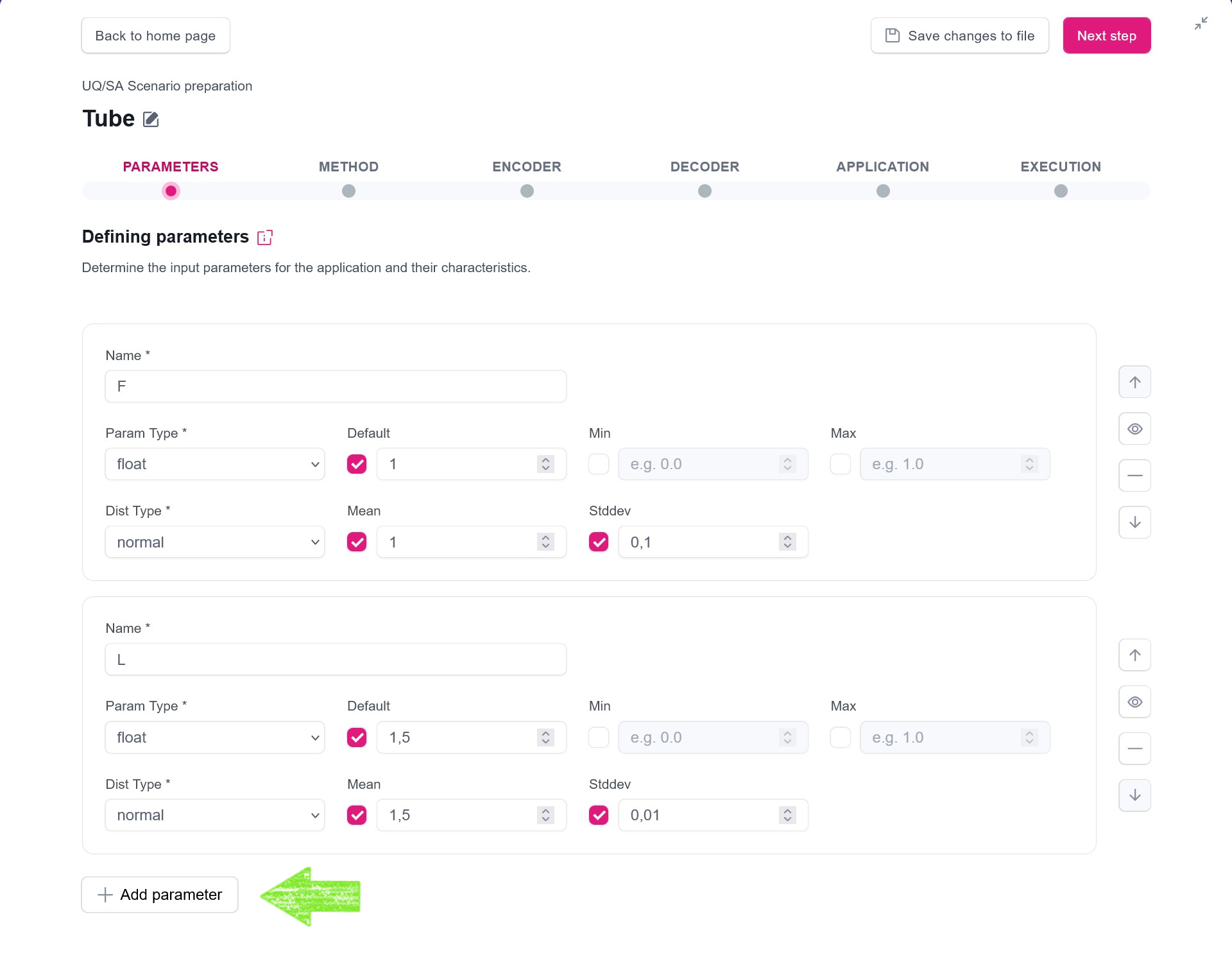
Tip
The provided configuration is simply a starting point. Feel free to explore the model and its uncertainty by tweaking default parameter values or by adjusting and substituting the suggested distributions.
Tip
For detailed information about the Parameters please see the documentation.
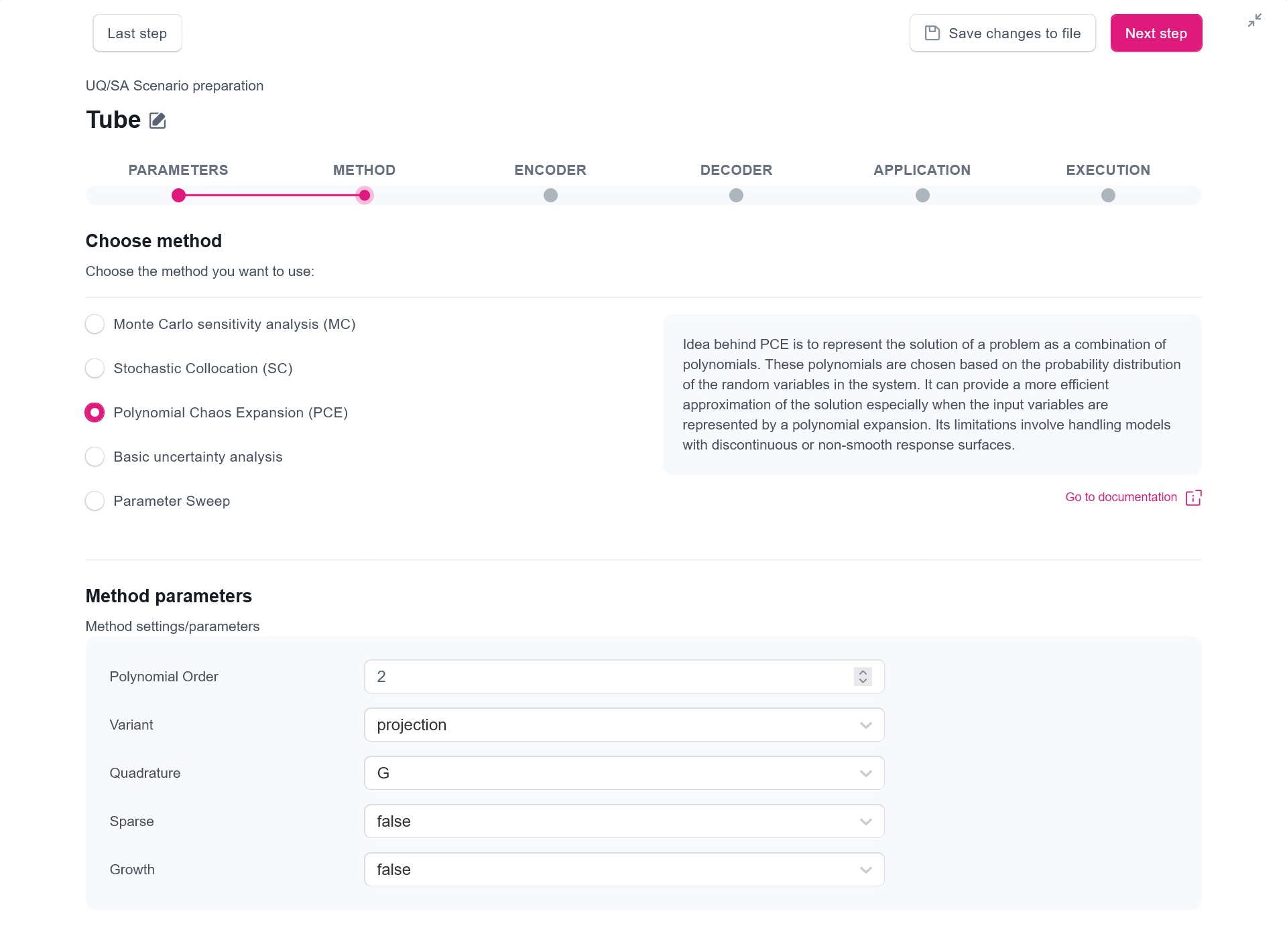
Step 2. Method
Depending on the aim of our UQ and SA studies, model characteristic and given the computational limitations (e.g., amount of CPUHours we want to spend on computations), we can select and then configure one of the provided methods.
For our example analysis, we will select Polynomial Chaos Expansion (PCE) method, with the default configuration. PCE is a robust instrument that can be used for both UQ and SA and typically provides good performance. For our use-case, the polynomial order value set to 3 will allow getting quite precise results with reasonable computational time. For testing purposes, you may set this value to 2, which will significantly decrease the number of computed evaluations.
Tip
For detailed information about the methods please see the documentation.
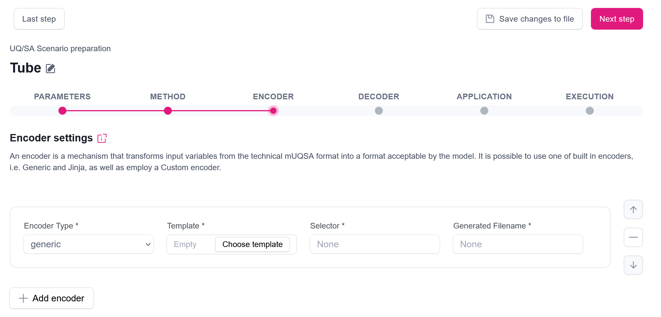
Step 3. Encoder
In order to execute individual model evaluations with the sampled parameters, mUQSA employs a concept of Encoder. The encoder takes the generic values from samplers and transfers them to the parameters passed to the executed model.
mUQSA currently provides two built-in encoders, namely Generic and Jinja, but a user can also provide its own decoder or even combine many encoders into a multi-encoder.
Since the Tube Deflection model takes a simple text file (JSON) as an input and there is no need to do any complex transformations, in our case, the Generic encoder is fully sufficient.
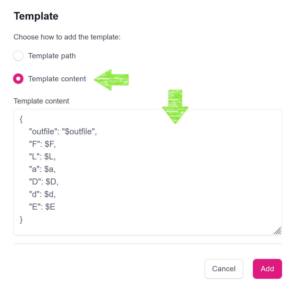
To configure the actual way how the encoder translates sampled parameters into the application input parameters, we need to provide a template. The content of the template for Tube Deflection looks as follows:
{
    "outfile": "$outfile",
    "F": $F,
    "L": $L,
    "a": $a,
    "D": $D,
    "d": $d,
    "E": $E
}
As you can see,
the template uses $-prefixed placeholders that will be substituted by the corresponding value of sampled parameter,
defined in the mUQSA parameters section.
To illustrate it better, let’s see how an example generated file can look for a single sample after the stage of sampling:
{
  "outfile": "output.json",
  "F": 1.03,
  "L": 1.49989,
  "a": 0.79,
  "D": 0.81,
  "d": 0.1,
  "E": 200000
}
The template can be provided in two ways: by entering a path to a template file available on a cluster, or by pasting the content of a template directly into the portal. Likely the second option is more convenient for small-sized templates, thus we will use it here. Firstly, we need to click Choose template button embedded in a Template text box. Once clicked, a new modal window opens, which, after selecting the Template content option, allows us to paste the template.
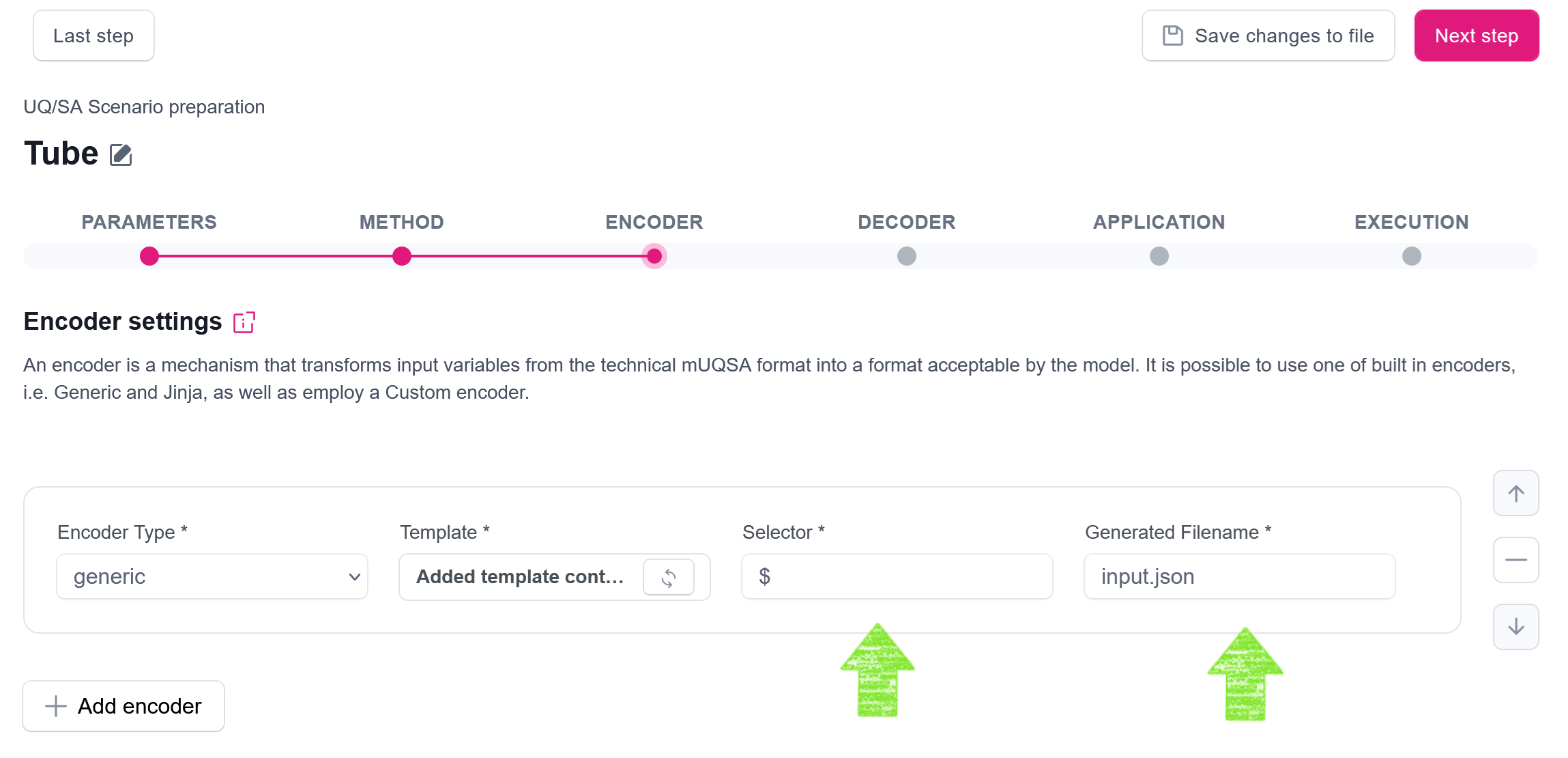
After clicking the Add button, the new template is assigned to the encoder. However, we need to complete this encoder configuration with two easy steps, namely
- we need to provide information what selector is used in placeholders in the provided template - in our case it is
$, - we need to specify a name of a file to which an encoder will save the generated input files after substitution made in the template - we will use
input.json.
Tip
For detailed information about the encoders please see the documentation.
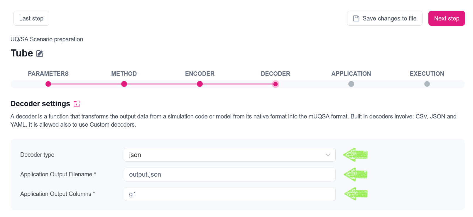
Step 4. Decoder
Decoder plays an analogical role to Encoder, but on the other side of the evaluation of the model: it takes the output generated by the model and transforms it to the form supported by mUQSA.
There are a couple of predefined decoder types, including csv (for parsing CSV files), json (for parsing JSON files) and yaml (for parsing YAML files). Additionally, it is possible to provide a custom decoder.
Let’s see how an example output from our model looks:
{"g1": -8.198586660713615e-06, "g2": -1.6483515629784663e-05, "g3": 1.6707539685614918e-05}
You can easily note that the format of this file is JSON, with 3 key-value pairs: g1, g2, g3.
Our quantity of interest is g1 (vertical deflection), which we would like to pass to mUQSA for further analysis.
Since our model generates a JSON file, the selection of json encoder type will be the most natural.
Obviously, we also need to define from which file the output data should be readout.
Finally, in order to pull values of g1 from the output files, we need to express that g1 values constitute the column we are interested in.
Note
In the presented example, since the JSON file is only one level depth, we reference the key simply by writing g1,
but it is also possible to handle structs of more complex JSON files and reference nested keys.
Tip
For detailed information about the decoders please see the documentation.
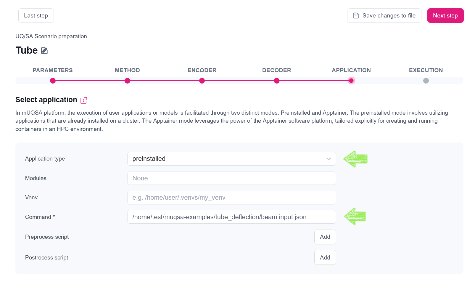
Step 5. Application
This step allows us to specify model for the evaluation. Our Tube Flow model has already been installed on a cluster, so we need to refer to it. Since the model is self-contained and has no particular dependencies, we just provide:
- Application type: preinstalled
- Command:
/home/test/muqsa-examples/tube_deflection/beam
The rest of the application configuration can be left empty.
Tip
For detailed information about the application configuration please see the documentation.
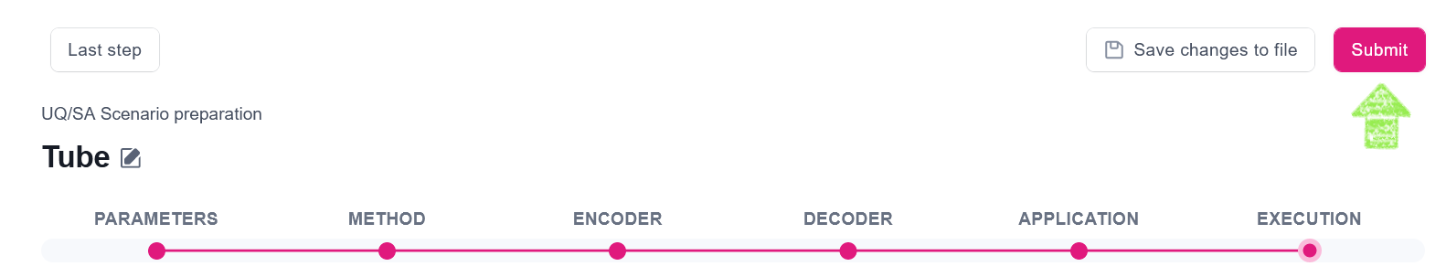
Step 6. Execution
Finally, in the Execution step, we need to specify how our UQ/SA scenario should be executed.
Info
Essentially, mUQSA is able to automatically adjust resource requirements to a certain scenario, ensuring efficient usage of resources, and taking into account the general preferences of a user.
This is how Execution configuration can be setup for the execution of our Tube Deflection model:
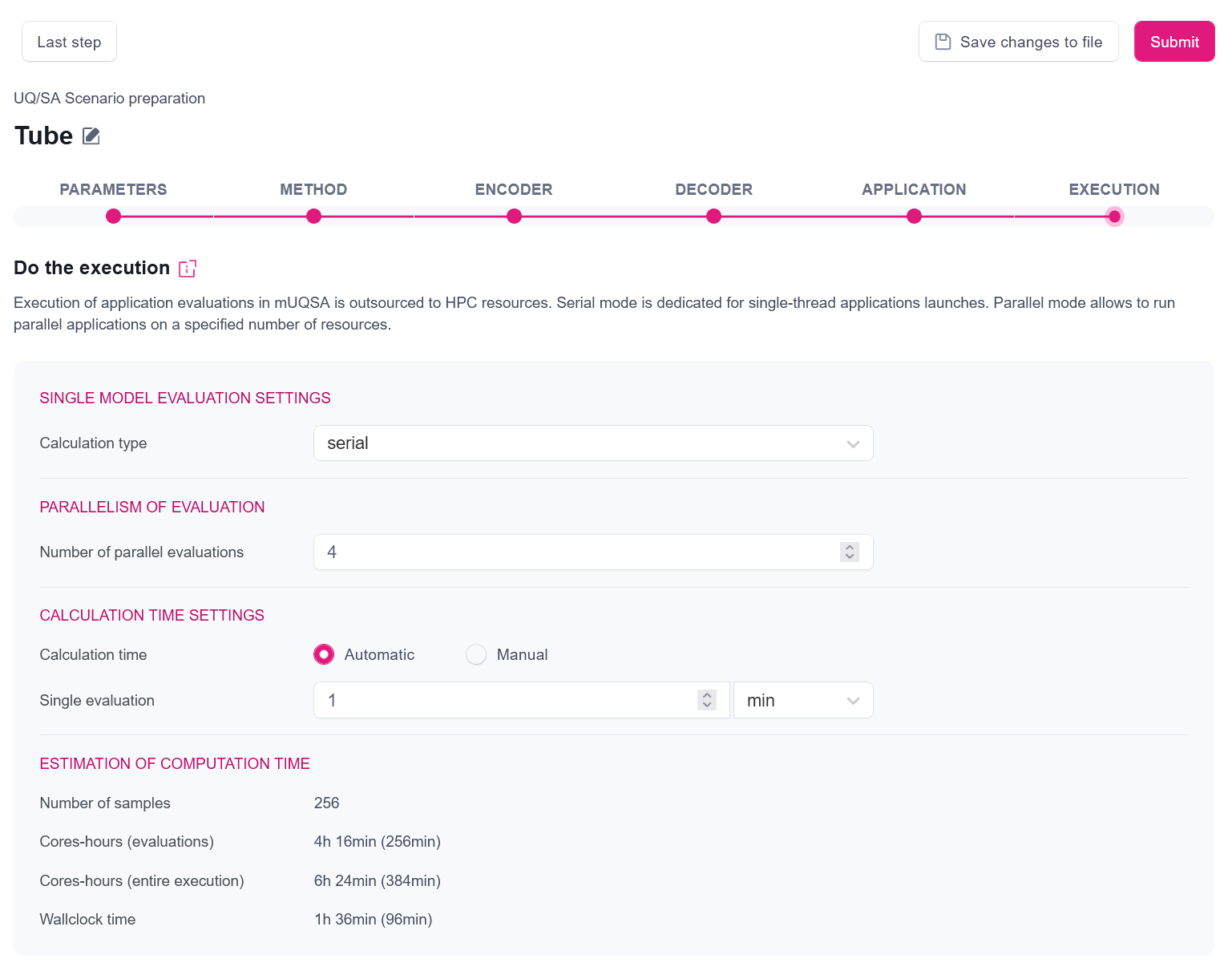
mUQSA gives quite powerful options here, so let us describe them quickly before we explain the individual settings from the screenshot.
The first section Single model evaluation settings allows us to define how a single evaluation of the application should be performed. We have two main options: serial (for execution of single-threaded applications) or parallel (for execution of parallel applications).
In the next section, Parallelism of evaluations we may define how many evaluations of a single model should be run in parallel.
Calculation time settings allow configuration of the wall clock time for the execution of scenario. A nice feature of mUQSA is that for some algorithms it can automatically predict the execution time of an entire scenario (with a some safety margin) based on the provided execution time of a single evaluation.
The last element presented in the view is the calculated prediction of a number of required evaluations and an estimation of resource consumption expressed in core-hours (for both evaluations only and entire execution) and wall clock time.
Having this background information, we can move to the explanation of the proposed settings.
- Since Tube Deflection is a simple, non-parallel code, we have selected the serial execution.
- By setting the Number of parallel evaluations to 4, we instruct the system to run up to 4 evaluations in parallel.
- The automatic setting of Calculation type, available for the selected algorithm, allows us to define time requirements only for a single evaluation of a model, leaving the calculation of the actual execution time needed for the inferred number of evaluations to mUQSA.
- Requested Single evaluation time is set here to 1 min.; this value, along with the number of parallel evaluations and the algorithm specificity, allow us to calculate cores hours needed for the evaluations and estimate an upper limit for both cores hours and the wall clock time for the entire execution (including not only evaluations, but also sampling, analysis and supplementary operations) As a matter of fact, 1 min. is far too long for the evaluation of our model, but in the real world scenarios we can expect much longer times.
- In the Estimation of computation time section, we can find some technical information about the planned execution, including a number of samples that will be evaluated, core hours, which likely be needed (for evaluation and for entire execution), and the calculated wall clock time, with a bit of safety margin, which our computations may take, and that will be passed to Slurm scheduling system in order to reserve computational resources for a sufficient period.
Tip
For more information about the configuration of execution, see the documentation.
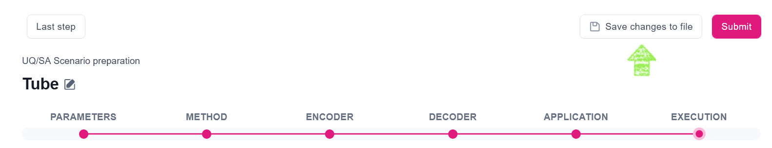
Saving configuration
mUQSA provides the possibility to save the configuration prepared in the wizard to a file, so it can be loaded later on for a new task. Configuration (completed or not) can be saved at each step using the dedicated button:
Running scenario (QCG-Portal)
Having scenario configuration prepared, we can schedule a new task for its execution by clicking the Submit button:
The confirmation of the submission is a modal window, which allows us to switch directly to QCG-Portal to track the progress of the submitted task execution or to submit another task.

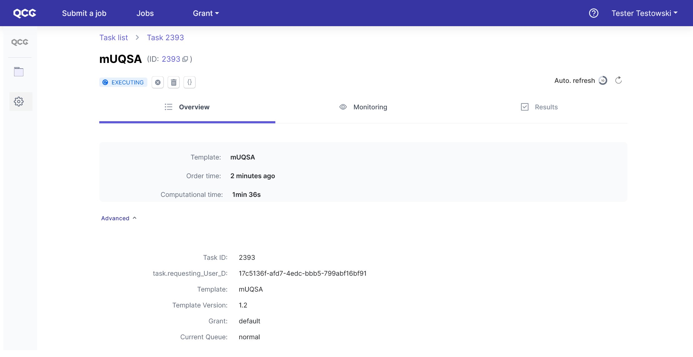
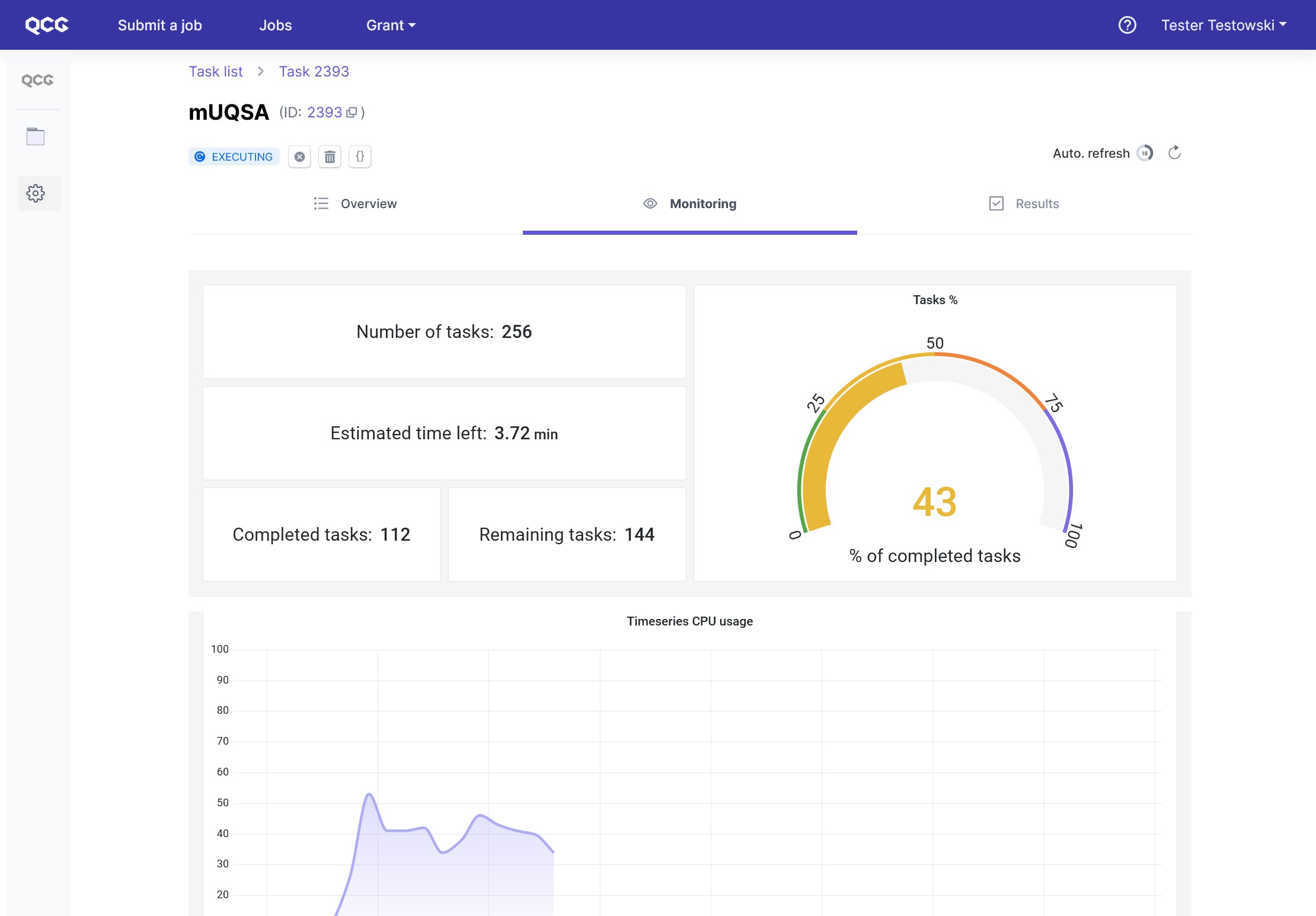
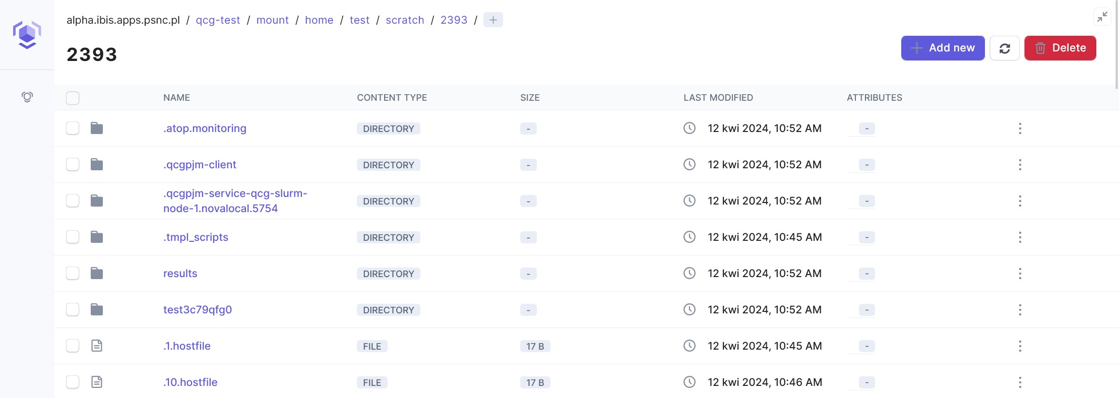
When we click on See the details of submitted job, we are moved directly to the task’s execution details in QCG-Portal. We can check the basic information on the task as well as monitor the execution progress. With built-in remote filesystem browser, we also are able to access working directory on a cluster during the task’s runtime to see logs or other files it produces.
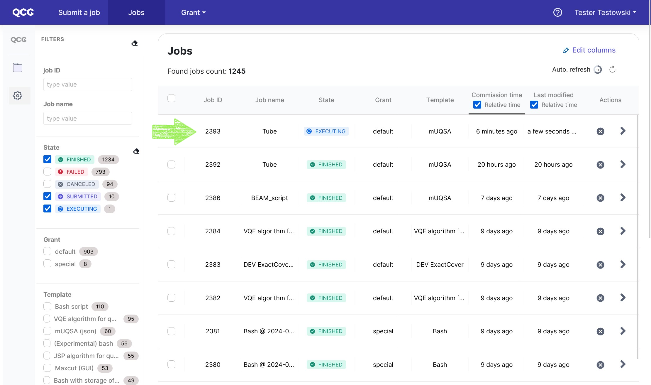
When we click on Jobs in the top menu, we are redirected to the list of submitted tasks. It is not difficult to spot the just submitted mUQSA task. In order to get back to its details, we need to use a dedicated action button “>”.
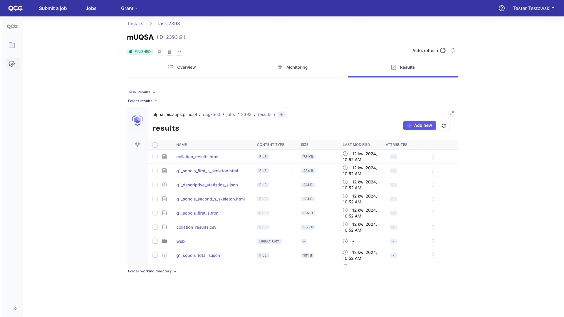
Once the task is finished, the Results tab became active, thus we can switch to it.

The pivotal element is here an interactive html web-page, which can be enlarged with the dedicated button. We will describe it in the next section. Additionally, via build-in remote filesystem explorer, users have access to the results in a raw form.
Analysis of results
mUQSA for the analysis of results creates a dedicated webpage. The content of the page varies from method to method or model to model, but it has some common elements, which we will firstly try to briefly outline based on the results obtained.
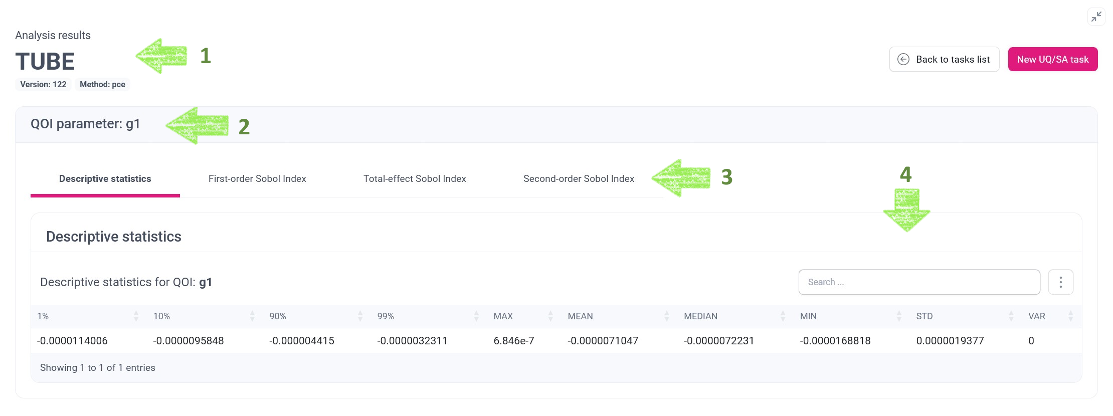
Let’s see what the green arrows indicate:
- High-level information about the analysis, including name of the analysis, version of the mUQSA template that has been used and the applied UQ/SA method.
- List of sections for one or many Quantities of Interests (QoIs). In the presented case, there is only a single section for g1 QoI.
- Number of tab panes for different kinds of statistics generated by the selected mUQSA method for a given QoI.
- Panel presenting statistical data in a form adjusted to the selected statistic.
Having this basic knowledge, now we will move to the examination of the Tube Deflection UQ/SA results.
Tip
For details on the mUQSA analysis function, see the documentation.
Descriptive statistics
The aim of Descriptive statistics is to provide general information about the uncertainty of the model. Consequently, the presented information includes the main statistical moments for the analysed QoI.
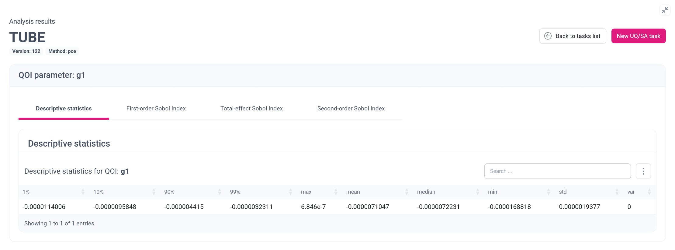
Since our model generates scalar data, our presentation is limited to a table with only a single row, and columns representing individual moments. In the case of vector QoIs, the table may significantly grow and the presentation of results will be more extensive.
For such complex cases, the table is equipped with a search field and a more button that offers both the ability to show or hide individual columns and to retrieve data stored in the table in different formats.
Sobol Indices
Sobol Index is a measure that allows to discover how the uncertainty of model parameters influences the output uncertainty. The result of Sobol’s analysis is a list of percentage values that displays a contribution of individual or combined input parameters variance on the variance of the results.
First-order Sobol Index displays the contribution of uncertainty of individual parameters on the output uncertainty. mUQSA presents this index in both graphical and tabular way.
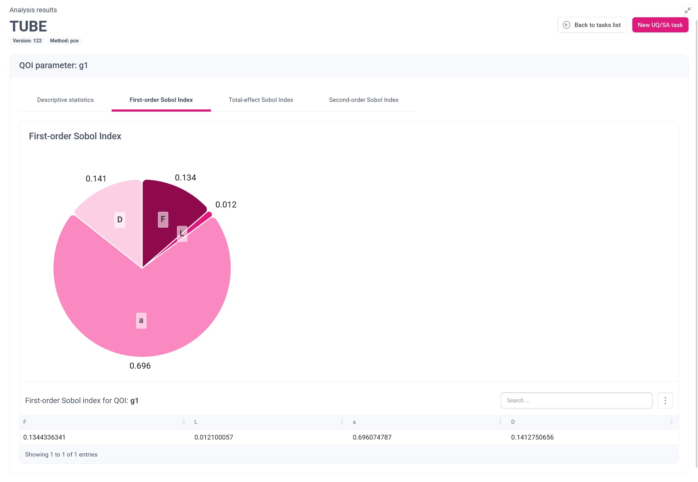
It is clearly visible that for the examined model, the parameter whose uncertainty has the greatest impact on QoI g1 is a (position of the force), next are D (external diameter of the tube) and F (the strength), whose impact is almost the same, and finally L (the length of the tube), with the lowest contribution.
Total-effect Sobol Index provides information about the complete contribution of input parameters uncertainty on the output uncertainty, including all interactions of a given parameter with other parameters. The presentation of Total-effect Sobol Index is analogous to the presentation of First-order Sobol Index.
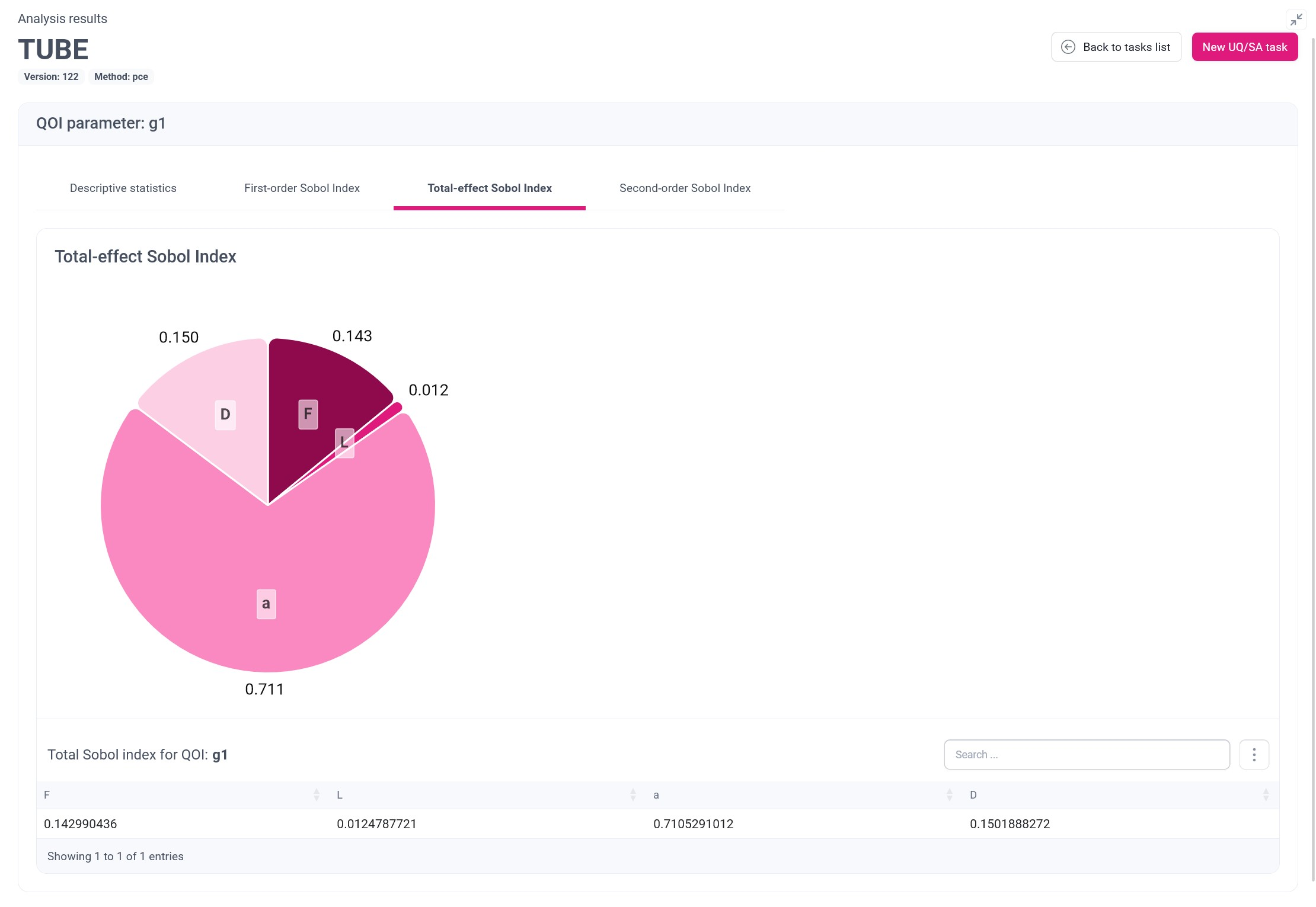
It can be noted that the relative contributions are very similar to the previously presented First-order Sobol Index, however, their absolute values are higher, which is a result of some interactions between the parameters. Frankly speaking, in this model, the uncertainty resulted from the interactions is not so high, but in other models it can have much more impact.
Second-order Sobol Index allows discovering uncertainty caused by interactions between pairs of parameters. mUQSA displays this metric in a form of two-dimensional table, where the value at the crossing of the column and row indicates the uncertainty contribution resulting from the interaction between the corresponding parameter from the first column and the first row.
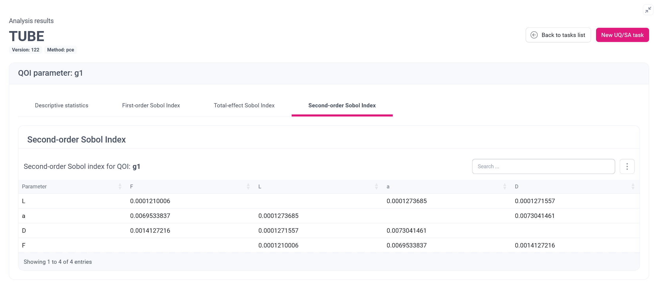
Keeping in mind the results from the two previous types of Sobol indices, where we have discovered that the uncertainty caused by all interactions between parameters is rather low, it is not a surprise, that the uncertainty caused by the interactions between only the individual pairs of elements must be also low. Nevertheless, some hypothetical analysis can be made, e.g. we can discover that the interaction between a and D is more significant in terms of uncertainty than the interaction between L and F.
Acquiring raw data
In addition to graphical and tabular presentation of data, mUQSA gives users the option to access the generated data in raw format. This is especially important for advanced scenarios where further analysis in external software may be required.
The data can be accessed via embedded file explorer on the Results view, from which a user can display or download files.