Lotka Volterra (vector QoI)
Introduction
In this tutorial, we will show how the mUQSA platform can be used for Uncertainty Quantification and Sensitivity Analysis of an example Lotka Volterra (prey-predator) model, which generates vectorised results.
This tutorial will also demonstrate the following two mUQSA features:
- how to configure UQ/SA of a model delivered in a form of an Apptainer (aka Singularity) image,
- how to use a custom decoder to alter the model’s output before it is analysed.
Description of a Lotka-Volterra model
Consider the following scenario: We are investigating the behavior of a predator-prey system using the Lotka-Volterra model, which describes the dynamics between predator and prey populations in a simplified ecosystem.
The Lotka-Volterra model, proposed by Alfred J. Lotka and Vito Volterra in the early 20th century, consists of a set of ordinary differential equations. It characterizes the interactions between two populations: predators and their prey. The model incorporates the following assumptions:
The prey population grows exponentially in the absence of predators.
The predator population declines exponentially in the absence of prey.
The rate of predation is proportional to the product of the predator and prey populations.
The mathematical representation of the Lotka-Volterra model is as follows:
$$ \frac{dx}{dt} = \alpha x - \beta xy $$ $$ \frac{dy}{dt} = \delta xy - \gamma y $$
Where:
- $x$ represents the prey population,
- $y$ represents the predator population,
- $alpha$ is a growth rate of prey,
- $beta$ is a death rate of prey due to activity of predators,
- $gamma$ is a natural death rate of predators,
- $delta$ is a factor describing how many consumed prey produces a new predator.
In this showcase, we will explore model behavior over some $time$ and with a specific time $step$. We have also introduced some internal stochastic behavior into the model; this can be fine-tuned with the $amp$ parameter.
Our aim is to apply Uncertainty Quantification to the Lotka-Volterra model by considering a hypothetical scenario with real-world relevance. We introduce uncertainties in input parameters such as growth rates, predation rates, and interaction rates. By conducting simulations and Sensitivity Analysis, we will explore how these uncertainties impact the stability and behavior of the predator-prey system over a specified duration.
The primary output of our model will be the number of prey and predators, providing insights into the population dynamics and potential implications for ecological systems.
Due to its simplicity, the model will allow you to get familiar with basic UQ & SA concepts without any background in the field.
Note
In this tutorial we will present the usage of mUQSA deployed in our test environment, but the procedure outlined is universal in key aspects and easily applicable to other mUQSA instances.
Application preparation
In order to employ mUQSA for the UQ&SA of a specific application, you need to take care of the preparation of this app, so it can be executed on a cluster. The basic option is to install it on a cluster and then reference to it from mUQSA, while the other is to use Apptainer/Singularity image that already contains the application. In this tutorial, we will focus on the second option.
Creating Apptainer image
In order to employ mUQSA for the UQ&SA of a specific application provided in a form of Apptainer image, you need to ensure that the host and container can exchange all necessary data between each other.
Basically, it is on Apptainer’s image creator to take care of mounting the working directory into the proper place of the container, so the data generated at the sampling phase can be passed to models, and vice versa, the data generated by the models can be passed to the collocation and analysis steps.
Knowing that encoding and encoding steps, like the model evaluation itself, are performed inside the container, the image’s creator needs also to ensure that all data required for Encoder and Decoder are available from the image (templates, Python classes, etc.).
Note
In the default configuration of Singularity, the directories $HOME, /tmp,
/proc, /sys, /dev and $PWD are among the system-defined bind paths,
so the files under these directories are already available from the container.
Creating Lotka-Volterra image
In order to create the Apptainer image, you need to have the Apptainer tool. Depending on preferences, you may install and use Apptainer from your laptop or use the Apptainer from the cluster. In this instruction, we will assume the second option.
Log-in into the cluster
ssh test@test.clusterCreate an interactive job
srun -N 1 -n 1 --pty /bin/bashAll the code needed for the building of Lotka-Volterra example is available in the git repository. Once the job is started, you can get it with the clone command:
git clone https://gitlab.pcss.pl/muqsa/muqsa-examples.gitThe Lotka-Volterra example is available in the
./muqsa-examples/lotka_volterradirectory. Let’scdto that directory:cd muqsa-examples/lotka_volterraAlong with a bunch of different items in this directory, you can figure-out
lotka-vector.deffile. This is an Apptainer receipt that defines how the image should be built:Bootstrap: docker From: python:3.11.4-alpine3.18 %setup mkdir -p ${SINGULARITY_ROOTFS}/lotka mkdir -p ${SINGULARITY_ROOTFS}/workdir %files lotka-volterra-vector.py /lotka/lotka-volterra-vector.py requirements.txt /lotka/requirements.txt %post apk add --update alpine-sdk pip install -r /lotka/requirements.txt %runscript cd /workdir python3 /lotka/lotka-volterra-vector.py "$@"The content isn’t complicated, but in the context of mUQSA, a few elements are worth signaling:
- First, we pack the application’s model code
lotka-volterra-vector.pyandrequirements.txtinto the/lotkadirectory, so these files are available in a specific directory inside the container. - Second, we create
/workdirthat plays a role of a working directory for our application inside a running container; from/workdirwe start the application. - Third, we do not pack other files that may be required by mUQSA itself for encoding or decoding phases, like a custom decoder
lotka-decoder.pythat we will use in our example; such files are loosely coupled with the underlying application code, so they can be bound at runtime.
- First, we pack the application’s model code
To build the image from the
lotka-vector.deffile, you may use the provided helper scriptbuild_image.sh:./build_image.shThe process of building the image may take some time. Once it is done, the new
lotka-vector.sigmimage should appear in the current directory.
Opening mUQSA (QCG-Portal)
In order to set up the execution of UQ/SA scenario with mUQSA, please log into QCG-Portal, which offers the mUQSA service (please note that you can also be redirected automatically to QCG-Portal from other services where you are already logged in):

Once logged in, the main view of the portal is displayed. We can see here a list of our tasks submitted with QCG-Portal to the execution on a cluster. Click on the Submit new button to define a new task:
A template selection view is now displayed. Since we are interested in mUQSA, please look for the mUQSA template and click Submit a job on it to initiate definition of a mUQSA scenario.

Now a welcome page of the mUQSA platform is presented. It is convenient to switch to its full-screen version by clicking the appropriate icon in the top-right corner.

Scenario setup
Now we are ready to move to the essence of our UQ/SA scenario preparation.
mUQSA welcome page allows you to load an already prepared scenario definition from a file, to which it was previously saved, or to create a one from scratch. We will follow the second option by clicking Assign new task.

Step 0. Name
Before we start configuring the scenario, we need to give it a name. Only alphanumeric characters and underscore are allowed. For simplicity, we will call our scenario “Lotka”.

Once accepted, you will be redirected to the 6-step mUQSA wizard, which will help us to set up all aspects of the scenario configuration.
Step 1. Parameters
The parameters section allows us to define a sampling space for the input parameters to our model. Depending on the variability of an input parameter, we may need to define its name, type, probability distribution along with its settings, default value and bounds.
Info
Proper selection of parameter distribution improves convergence rates of UQ/SA algorithms. If you are not sure what distribution your input parameter comes from, then the uniform distribution may be the only reliable choice.
In the case of Lotka-Volterra model, we consider the following list of parameters:
| Parameter Name | Type | Distribution | Default Value |
|---|---|---|---|
| alpha | float | Uniform(0.1, 3.0) | 1.0 |
| beta | float | Uniform(0.1, 2.0) | 0.1 |
| gamma | float | Uniform(0.1, 2.0) | 0.5 |
| delta | float | Uniform(0.01, 0.9) | 0.03 |
| prey | float | None | 100 |
| predator | float | None | 25 |
| time | float | None | 3 |
| step | float | None | 0.01 |
| amp | float | None | 0.1 |
As you can see, some parameters (alpha, beta, gamma, delta) have the uniform distributions defined: UQ algorithms will sample these parameters from the given distributions. Other parameters (prey, predator, time step and amp) do not have distributions set up, so their default values will be used.
Definition of Parameters in mUQSA looks as follows (a new parameter can be added with Add parameter button):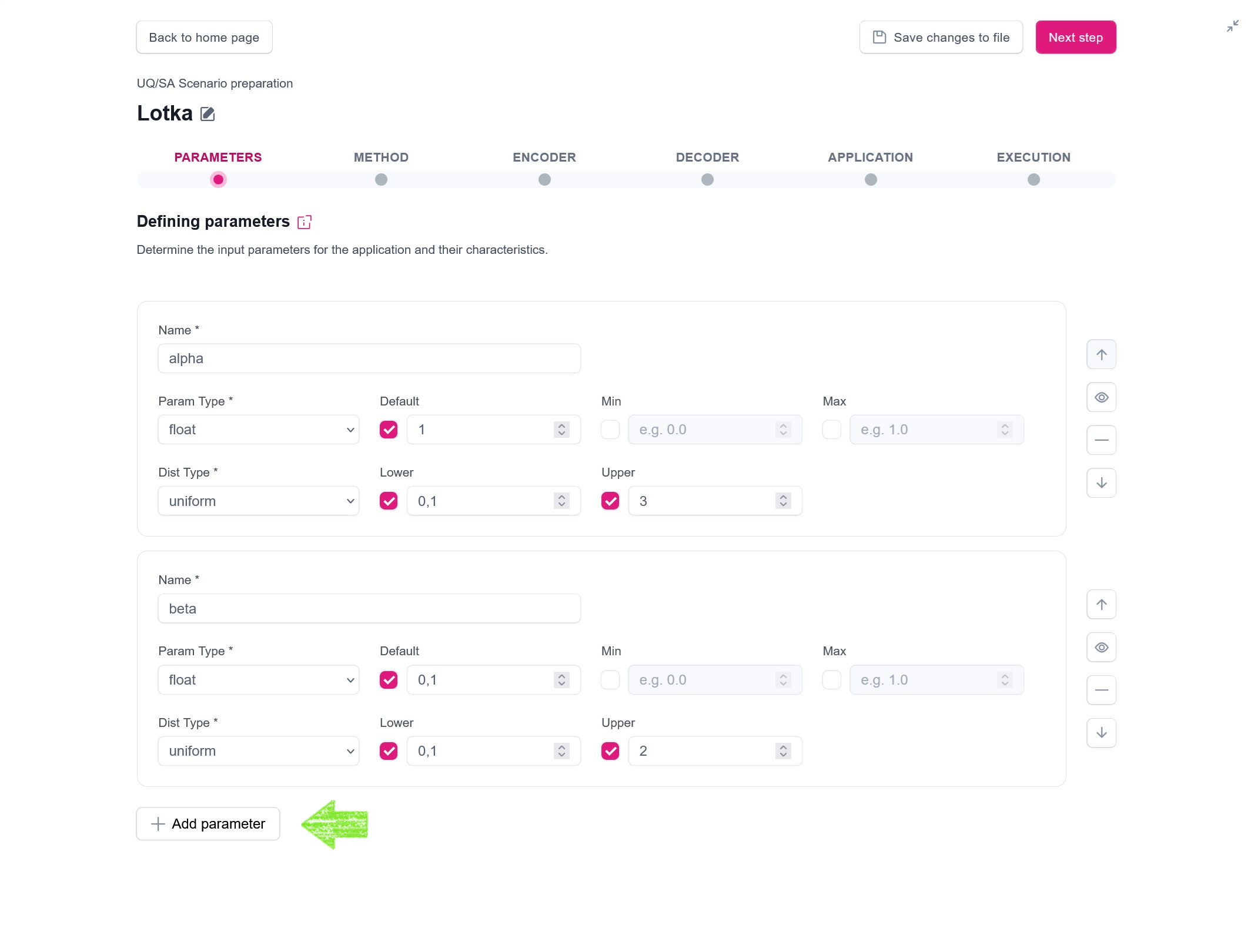
Tip
The provided configuration is simply a starting point. Feel free to explore the model and its uncertainty by tweaking default parameter values or by adjusting and substituting the suggested distributions.
Tip
For detailed information about the Parameters please see the documentation.
Step 2. Method
Depending on the aim of our UQ and SA studies, model characteristic and given the computational limitations (e.g., amount of CPUHours we want to spend on computations), we can select and then configure one of the provided methods.
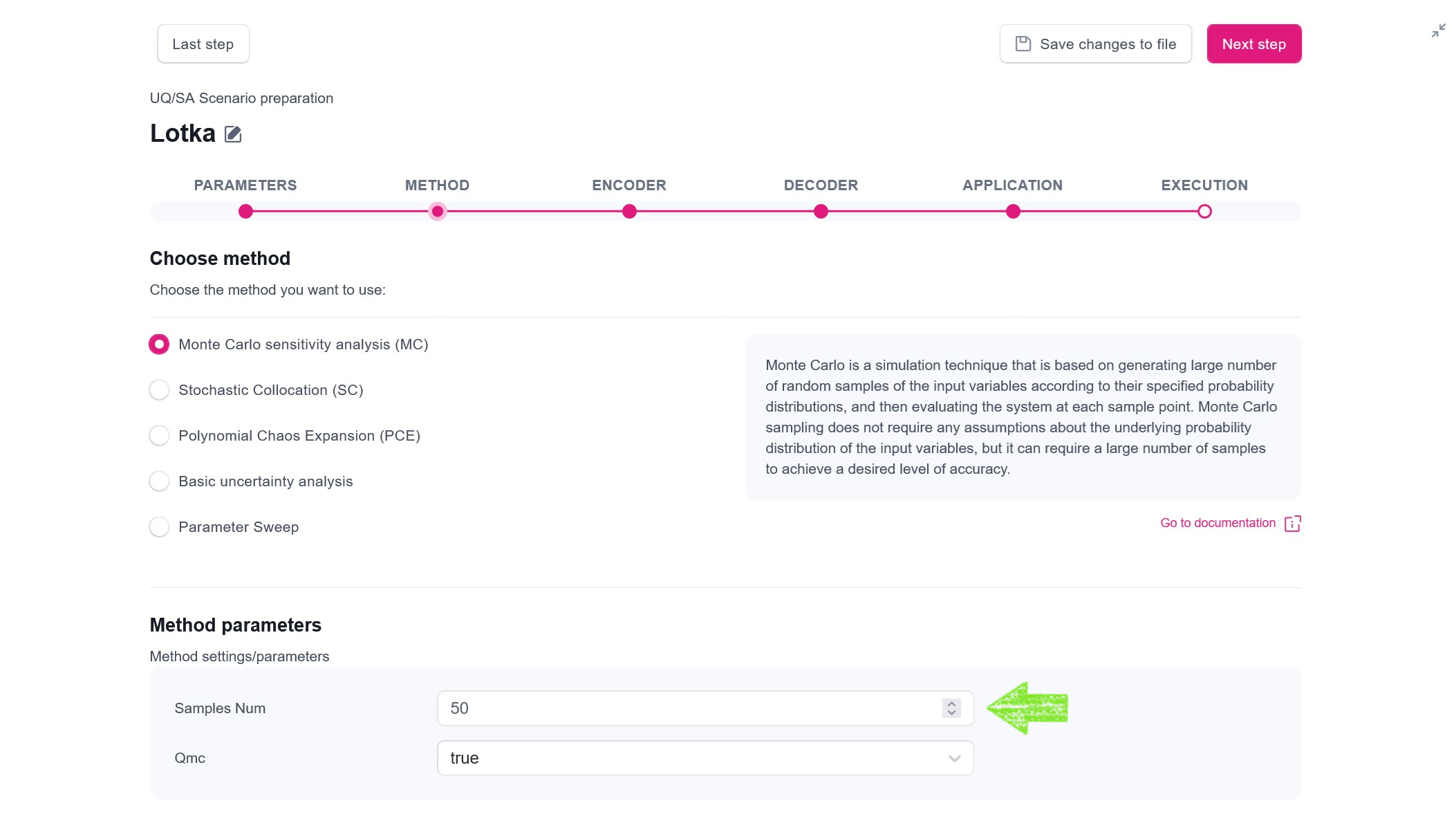
For this example analysis, we will use the Monte Carlo (MC) method, with the following configuration:
- number of samples generated by the method from an input random variable: 50,
- method variant: Quasi Monte Carlo (QMC)
Note
QMC algorithm uses Saltelli sampling plan to generate samples. Since QMC is usually more robust that pure MC, mUQSA uses QMC by default.
Note
We encourage you to try other methods and to play with their configuration.
Tip
For detailed information about the methods please see the documentation.
Step 3. Encoder
In order to execute individual model evaluations with the sampled parameters, mUQSA employs a concept of Encoder. The encoder takes the generic values from samplers and transfers them to the parameters passed to the executed model.
mUQSA currently provides two built-in encoders, namely Generic and Jinja, but a user can also provide its own decoder or even combine many encoders into a multi-encoder.
Our application to run needs only a single input file, with the following structure:
{
  "alpha": 1.2,
  "beta": 1.5,
  "gamma": 1.0,
  "delta": 0.3,
  "prey": 100,
  "predator": 25,
  "time": 3,
  "step": 0.01,
  "amp": 0.1
}
It’s apparent that this is a JSON file, which consists of some key-value pairs corresponding to the model’s parameters. For UQ, we are going to generate such files by substituting values with the sampled ones. Since the values can be put as they are, and there is no need to do any complex transformations, we will use the most basic, Generic encoder.
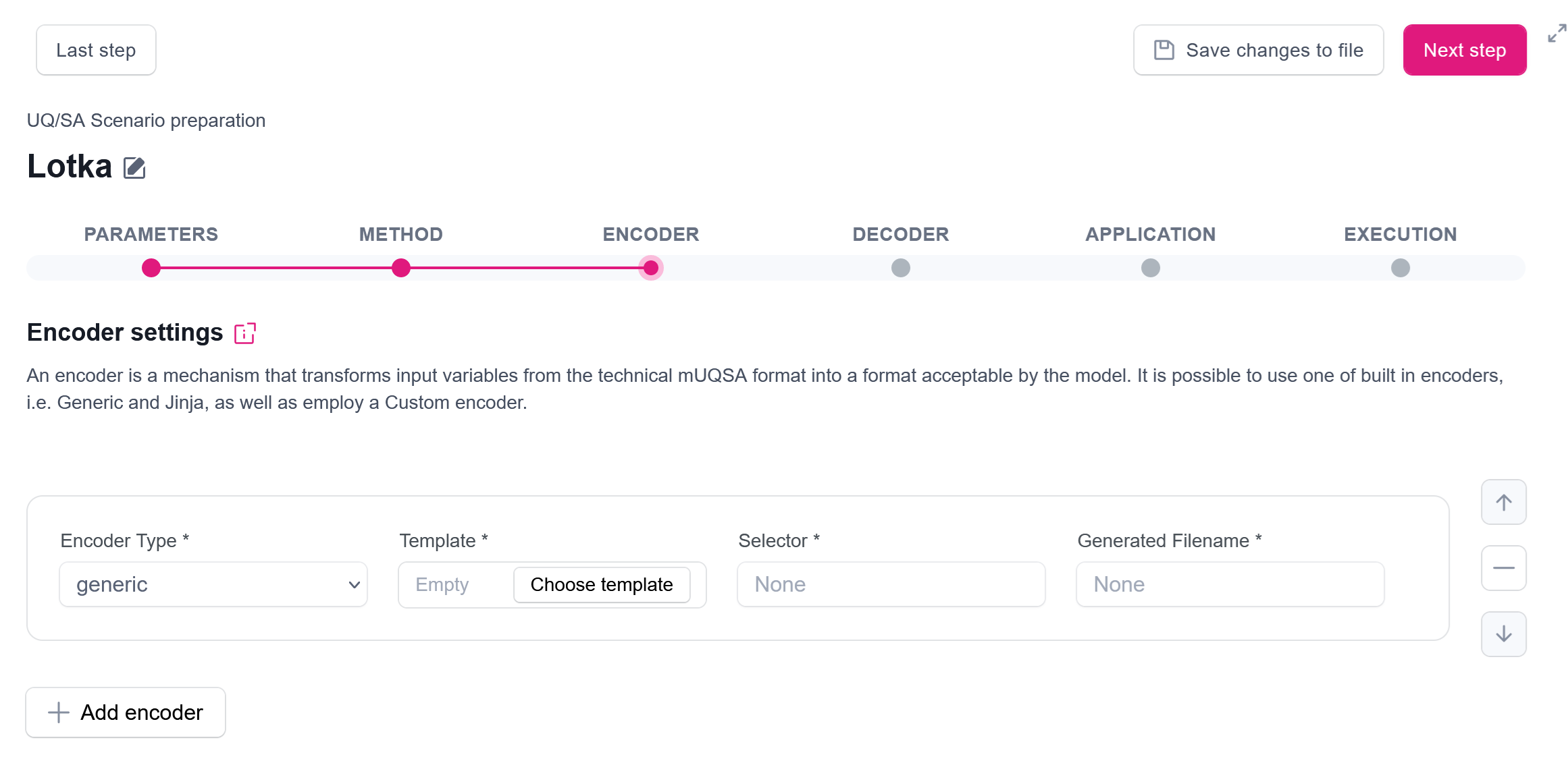
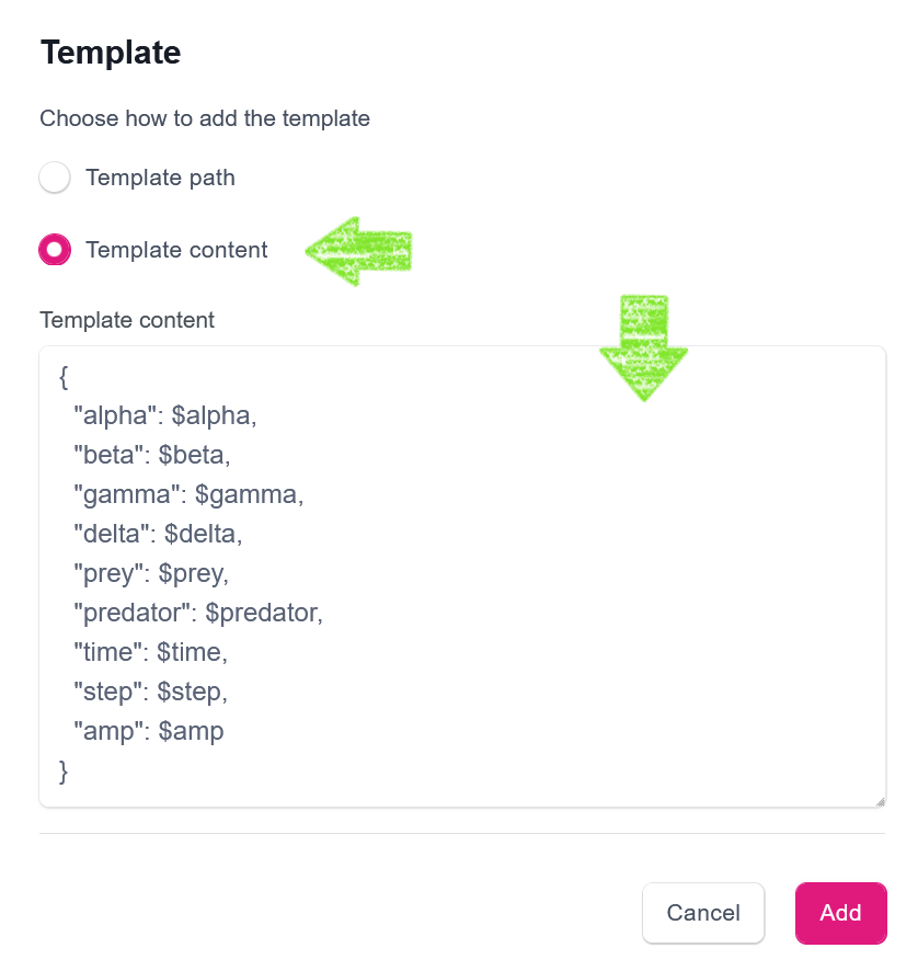
The Generic encoder translates sampled parameters into the application input form using a simple templating mechanism that replaces defined placeholders with the corresponding sampled values. Thus, for the Lotka-Volterra model, the template may look as follows:
{
  "alpha": $alpha,
  "beta": $beta,
  "gamma": $gamma,
  "delta": $gamma
  "prey": $prey,
  "predator": $predator,
  "time": $time,
  "step": $step,
  "amp": $amp
}
As you can see the template contains $-prefixed placeholders.
These placeholders will be substituted by the corresponding values of sampled parameters,
defined in the mUQSA parameters section.
The template can be provided in two ways: by entering a path to a template file available on a cluster, or by pasting the content of a template directly into the portal. Likely the second option is more convenient for small-sized templates, thus we will use it here. Firstly, we need to click Choose template button embedded in a Template text box. Once clicked, a new modal window opens, which, after selecting the Template content option, allows us to paste the template.
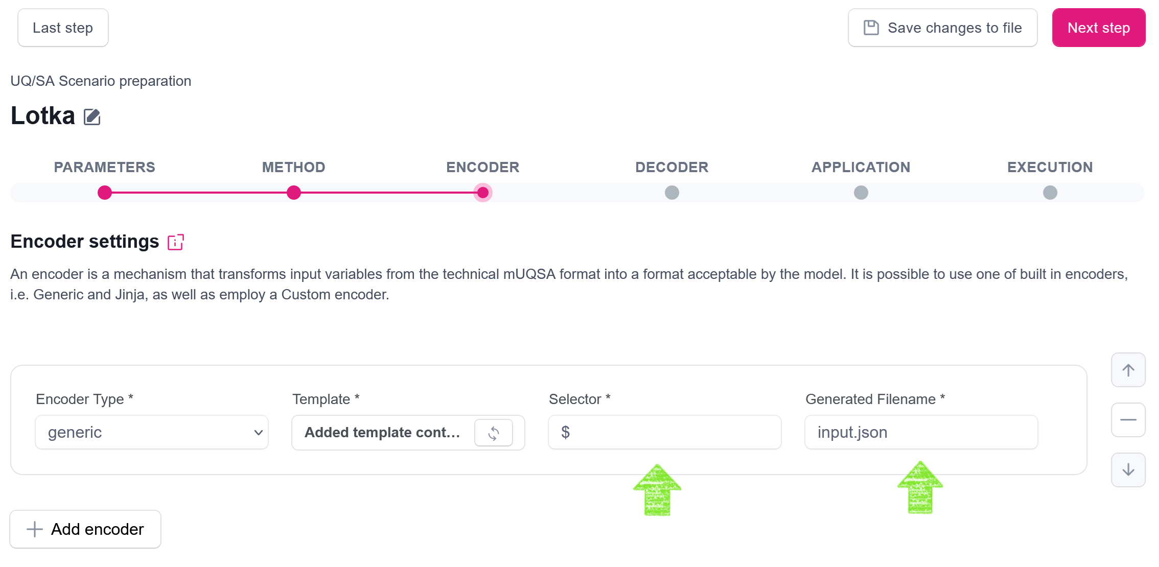
After clicking the Add button, the new template is assigned to the encoder. However, we need to complete this encoder configuration with two easy steps, namely:
- we need to provide information what selector is used in placeholders in the provided template - in our case it is
$, - we need to specify a name of a file to which an encoder will save the generated input files after substitution made in the template - we will use
input.json.
Tip
For detailed information about the encoders please see the documentation.
Step 4. Decoder
Decoder plays an analogical role to Encoder, but on the other side of the evaluation of the model: it takes the output generated by the model and transforms it to the form supported by mUQSA.
There are a couple of predefined decoder types, including csv (for parsing CSV files), json (for parsing JSON files) and yaml (for parsing YAML files). Additionally, it is possible to provide a custom decoder.
Our application code generates only a single output file called output.csv.
Let’s see how an example content of this file looks:
time,prey,predator
0.0,100.0,25.0
0.01,82.54997565089357,44.81855251838864
0.02,54.041382243682555,75.50177715356261
0.03,21.37373239806974,107.72471331865779
0.04,2.4561581556422993,125.35348168553966
0.05,0.30461518822362965,125.65943886420801
0.06,-0.006202565863006215,123.76084703461534
0.07,-0.00059691627919666,121.54785250415061
0.08,-3.338082403916639e-05,119.22158130110162
...
2.99,-3.2870509294035083e-32,0.49437211168130685
It’s quite apparent that the format of this file is CSV, with 3 columns: time, prey, predator.
We are interested in the analysis of prey and predator values in relation to time.
So, using the CSV decoder seems like the natural choice, right?
This is not a full truth, but let’s temporarily assume it is, for simplicity.
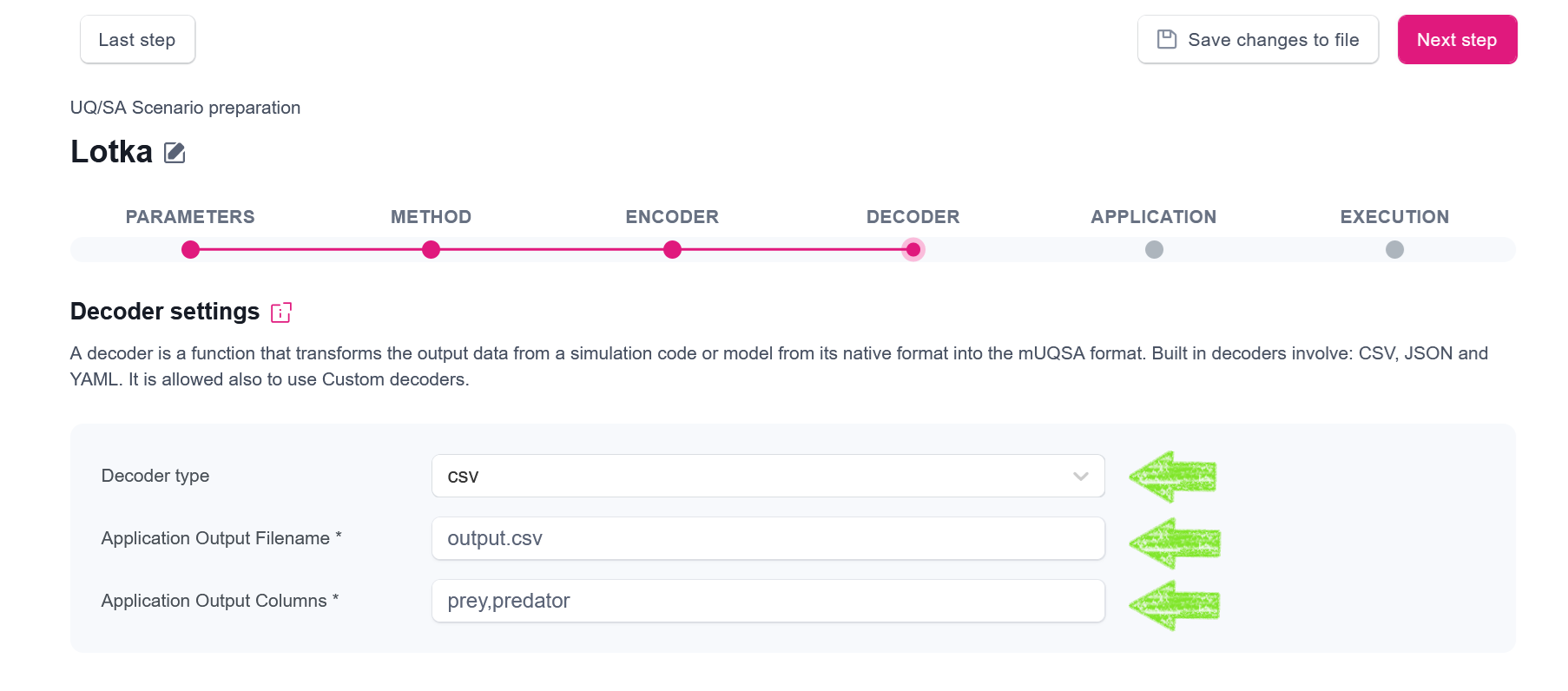
CSV decoder - basic
To set up the CSV decoder for our needs, we need to select it from the combobox, and then configure it as follows:
- Application ouptut filename should be set to
output.csv, as this is the name of a result file our application generates. - Application output columns should be set to
prey,predator, as these are our QoIs.
Custom decoder - advanced
We have said that the CSV decoder is not a perfect solution for our case, but why? The short answer is: because there can be an issue with the first row of data produced by our model. In the first row, the model outputs the initial values for prey and predator that are not sensitive to any sampled input. This may cause issues for some UQ algorithms (e.g. PCE) , which may generate strange statistics for this initial step. Therefore, we may slightly modify the CSV Decoder, so it will drop the first row.
To do so, the most simplistic way is just to copy the code of the original CSV decoder available in the EasyVVUQ repository
(easyvvuq.decoders.simple_csv.py), and slightly modify its code, so it will skip the 0-th observation.
The amendment decoder has already been prepared,
and it is available under the lotka.decoder.py filename in the lotka_volterra tutorial’s directory.
The only changes to its predecessor is the change of a decoder’s class name to SimpleCSVWithoutFirstLine and invocation of a next(reader) method that allows us to skip the first line.
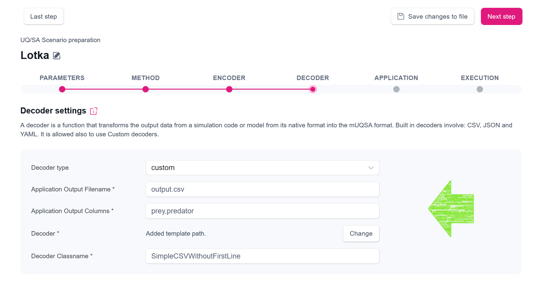
Having this information, we can configure our custom encoder, in the following way:
- Application ouptut filename should be set to
output.csv, as this is the name of a result file our application generates. - Application output columns should be set to
prey,predator, as these are our QoIs. - Decoder should be selected using the Template path option, where the Template path should be set to the location of the
lotka-decoder.pyfile in the container’s filesystem (the file’s location may need to be bound from the host; in our case it is in the user’s home directory, which is being bound automatically).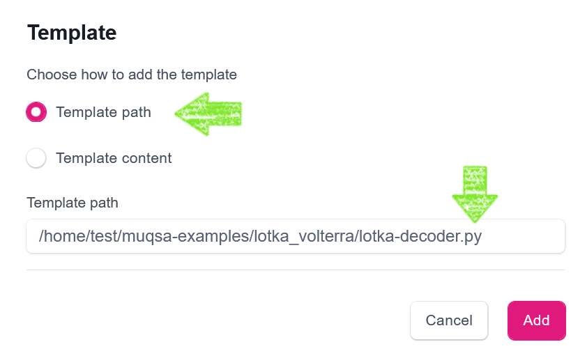
Selecting Custom decoder with file path - Decoder Classname should be set to
SimpleCSVWithoutFirstLine, as this is the class name of our decoder.
Tip
For detailed information about the decoders please see the documentation.
Step 5. Application
This step allows us to specify an application model for the evaluation. mUQSA allows us to work with the applications already installed on a cluster (preinstalled) as well as with the ones provided in the form of Apptainer images. As you already know, our Lotka-Volterra model is boundled into the Apptainer image, so we will demonstrate the second option here.
Assuming that the image with the application is already available on the cluster inside the /home/test/muqsa-examples/lottka-voltera/lotka-voltera.simg file
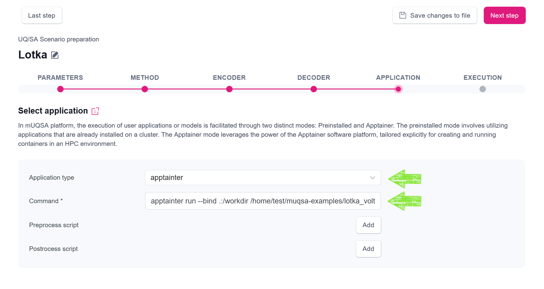
(regardless it was created or transferred there), to set up the application, we need to enter the following configuration:
- Application type: apptainer
- Command:
apptainter run --bind .:/workdir /home/test/muqas-examples/lotka_volterra/lotka-volterra.simg input.json
Please take note of two points on the Command:
- First, we bind the current directory
(the directory where the computations will be performed) to
/workdirin the container. This is because the container assumes that the data needing exchange between the host and container should reside in /workdir." - Second, we provide
input.jsonas an argument to the image.input.jsondenotes a file generated by the encoder for every set of sampled data. With each evaluation, the correspondinginput.jsonfile is passed to a singular model run.
Tip
For detailed information about the application configuration please see the documentation.
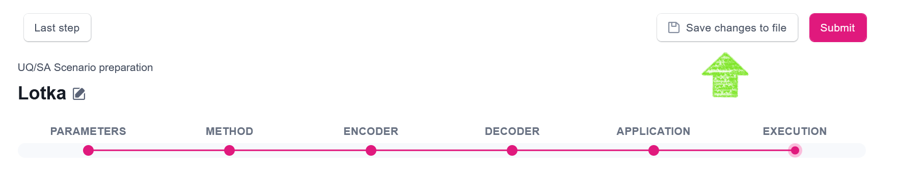
Step 6. Execution
Finally, in the Execution step, we need to specify how our UQ/SA scenario should be executed.
Info
Essentially, mUQSA is able to automatically adjust resource requirements to a certain scenario, ensuring efficient usage of resources, and taking into account the general preferences of a user.
This is how Execution configuration can be setup for the execution of our model:
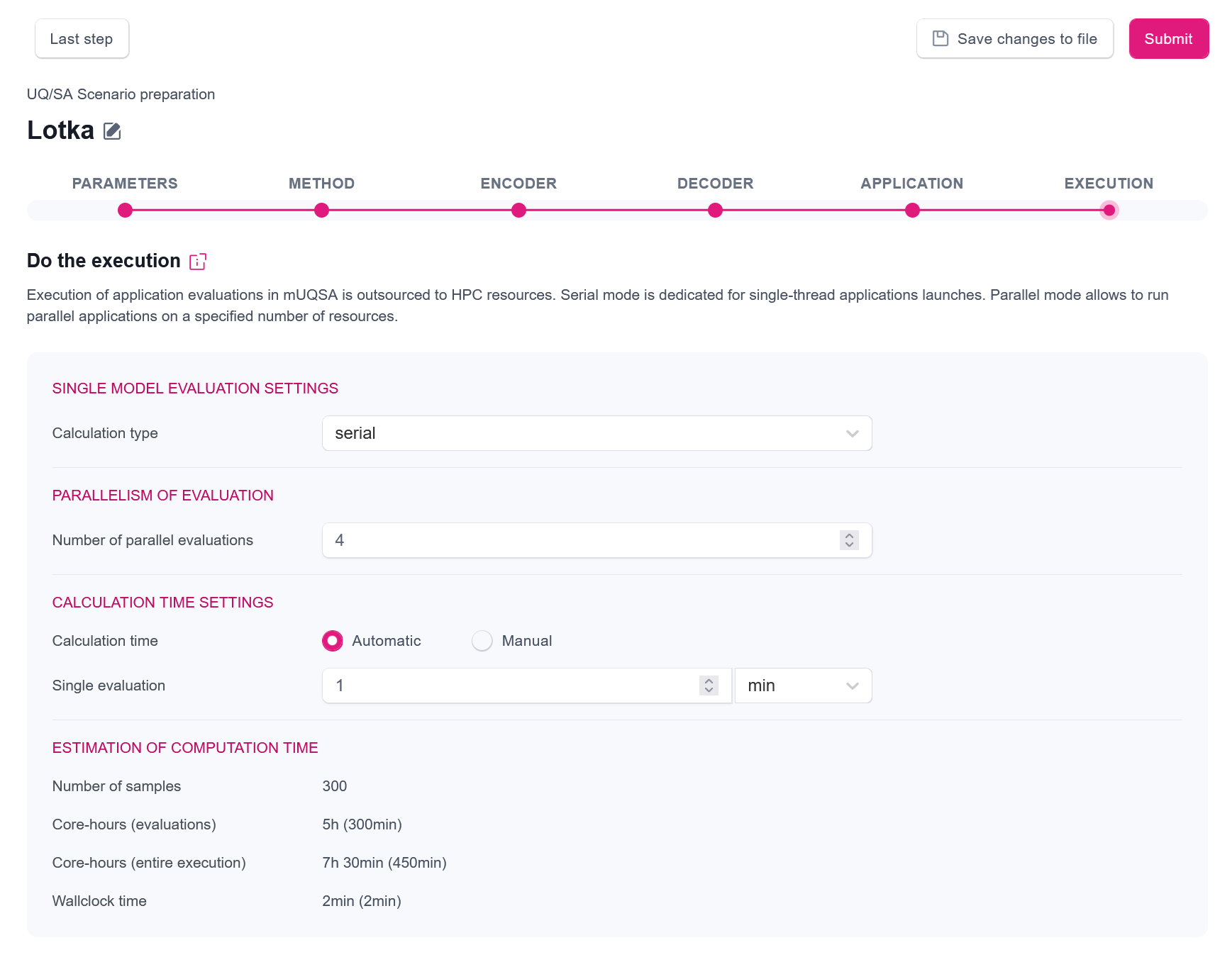
mUQSA gives quite powerful options here, so let us describe them quickly before we explain the individual settings from the screenshot.
The first section Single model evaluation settings allows us to define how a single evaluation of the application should be performed. We have two main options: serial (for execution of single-threaded applications) or parallel (for execution of parallel applications).
In the next section, Parallelism of evaluations we may define how many evaluations of a single model should be run in parallel.
Calculation time settings allow configuration of the wall clock time for the execution of scenario. A nice feature of mUQSA is that for some algorithms it can automatically predict the execution time of an entire scenario (with a some safety margin) based on the provided execution time of a single evaluation.
The last element presented in the view is the calculated prediction of a number of required evaluations and an estimation of resource consumption expressed in core-hours (for both evaluations only and entire execution) and wall clock time.
Having this background information, we can move to the explanation of the proposed settings.
- Since Lotka-Volterra is a simple, non-parallel code, we have selected the serial execution.
- By setting the Number of parallel evaluations to 4, we instruct the system to run up to 4 evaluations in parallel.
- The automatic setting of Calculation type, available for the selected algorithm, allows us to define time requirements only for a single evaluation of a model, leaving the calculation of the actual execution time needed for the inferred number of evaluations to mUQSA.
- Requested Single evaluation time is set here to 1 min.; this value, along with the number of parallel evaluations and the algorithm specificity, allow us to calculate cores hours needed for the evaluations and estimate an upper limit for both cores hours and the wall clock time for the entire execution (including not only evaluations, but also sampling, analysis and supplementary operations) As a matter of fact, 1 min. is far too long for the evaluation of our model, but in the real world scenarios we can expect much longer times.
- In the Estimation of computation time section, we can find some technical information about the planned execution, including a number of samples that will be evaluated, core hours, which likely be needed (for evaluation and for entire execution), and the calculated wall clock time, with a bit of safety margin, which our computations may take, and that will be passed to Slurm scheduling system in order to reserve computational resources for a sufficient period.
Tip
For more information about the configuration of execution, see the documentation.
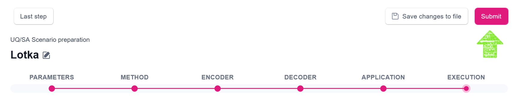
Saving configuration
mUQSA provides the possibility to save the configuration prepared in the wizard to a file, so it can be loaded later on for a new task. Configuration (completed or not) can be saved at each step using the dedicated button:
Running scenario (QCG-Portal)
Having scenario configuration prepared, we can schedule a new task for its execution by clicking the Submit button:
The confirmation of the submission is a modal window, which allows us to switch directly to QCG-Portal to track the progress of the submitted task execution or to submit another task.

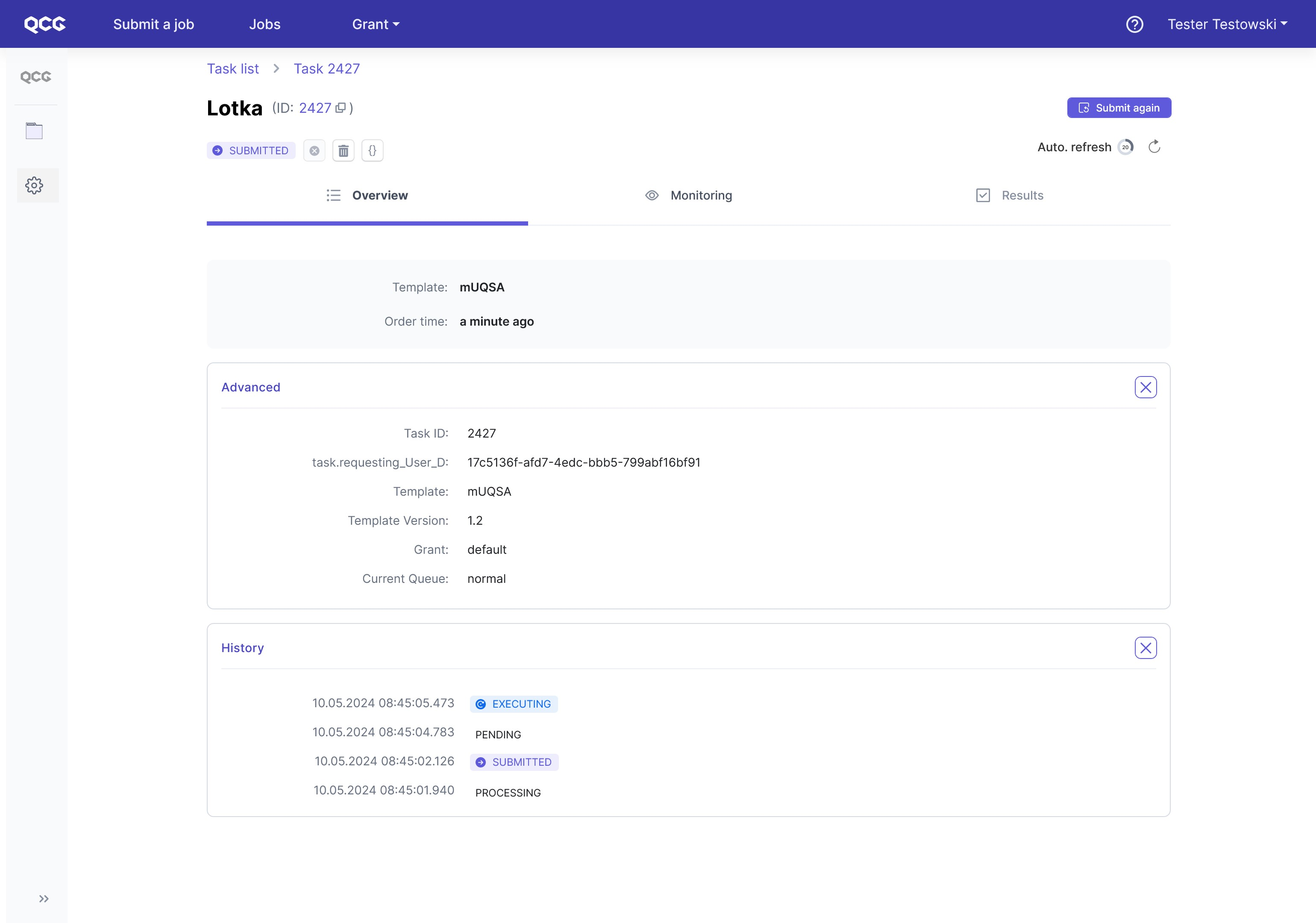
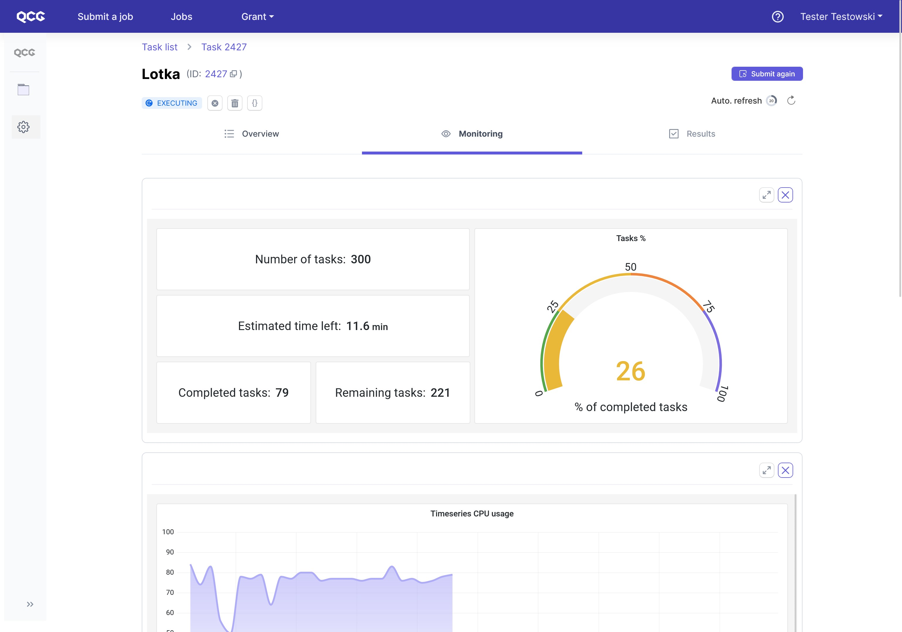
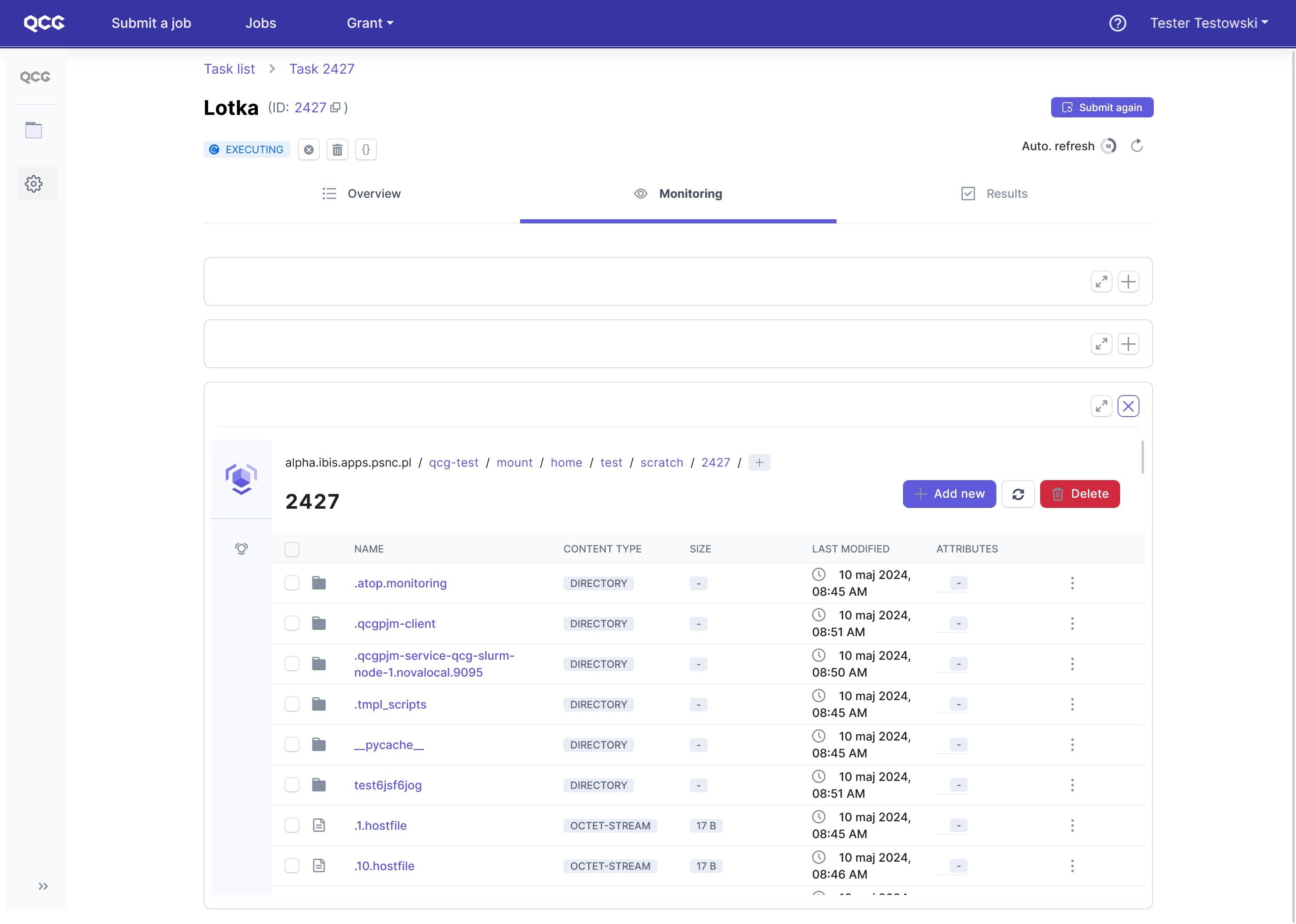
When we click on See the details of submitted job, we are moved directly to the task’s execution details in QCG-Portal. We can check the basic information on the task as well as monitor the execution progress. With built-in remote filesystem browser, we also are able to access working directory on a cluster during the task’s runtime to see logs or other files it produces.
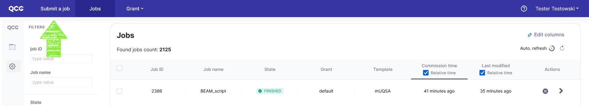
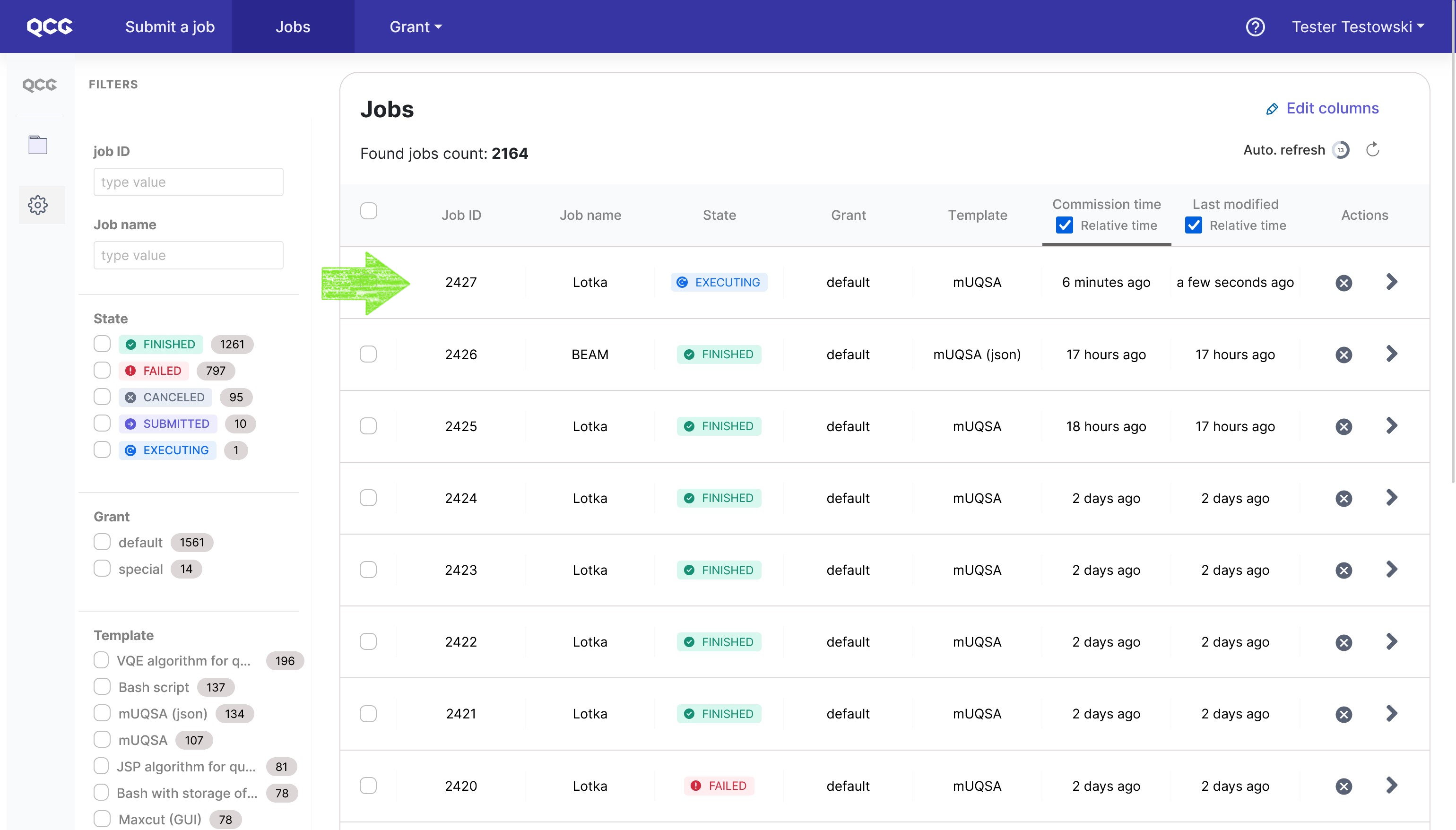
When we click on Jobs in the top menu, we are redirected to the list of submitted tasks. It is not difficult to spot the just submitted mUQSA task. In order to get back to its details, we need to use a dedicated action button “>”.
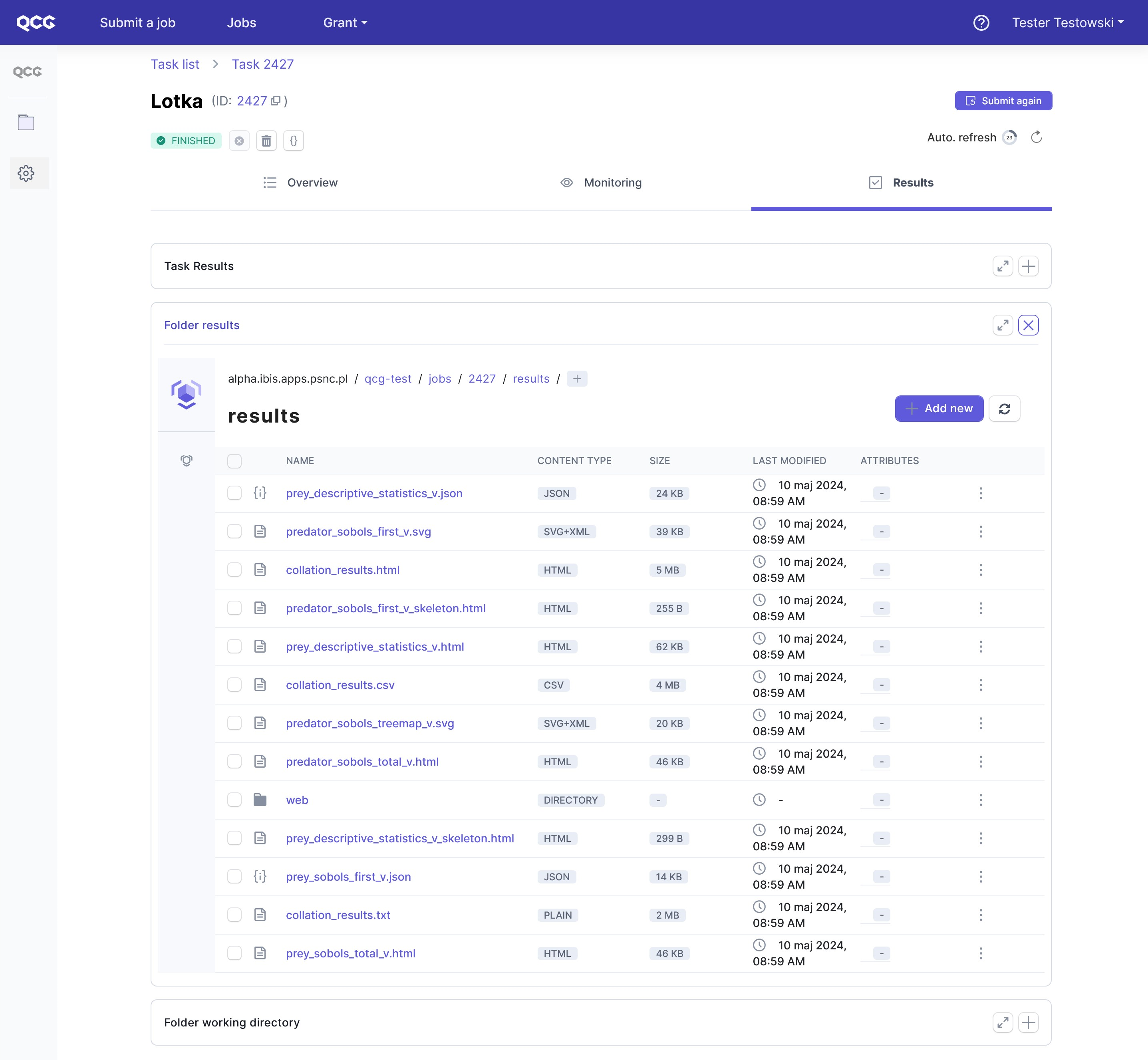
Once the task is finished, the Results tab became active, thus we can switch to it.
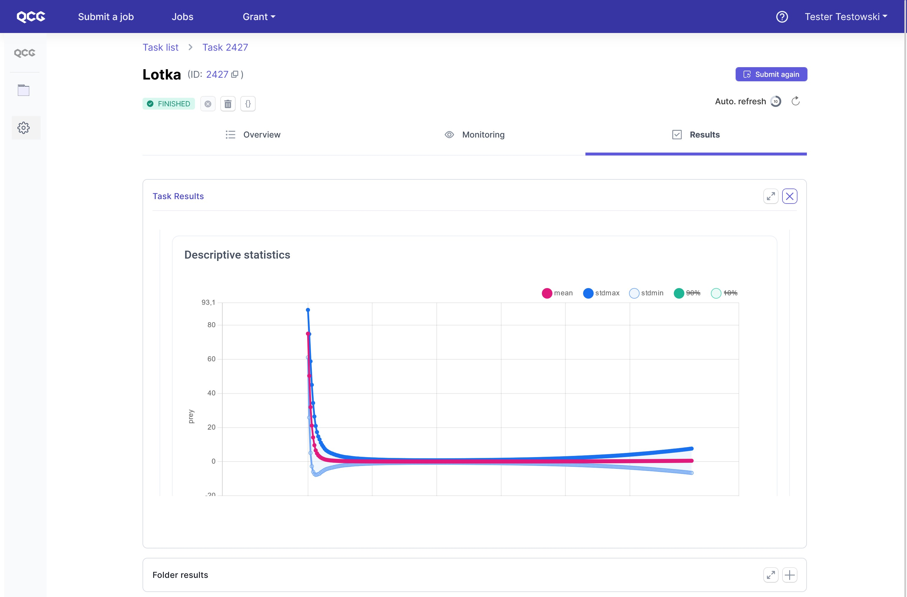
The pivotal element is here an interactive html web-page, which can be enlarged with the dedicated button. We will describe it in the next section. Additionally, via build-in remote filesystem explorer, users have access to the results in a raw form.
Analysis of results
mUQSA for the analysis of results creates a dedicated webpage. The content of the page varies from method to method or model to model, but it has some common elements, which we will firstly try to briefly outline based on the results obtained.
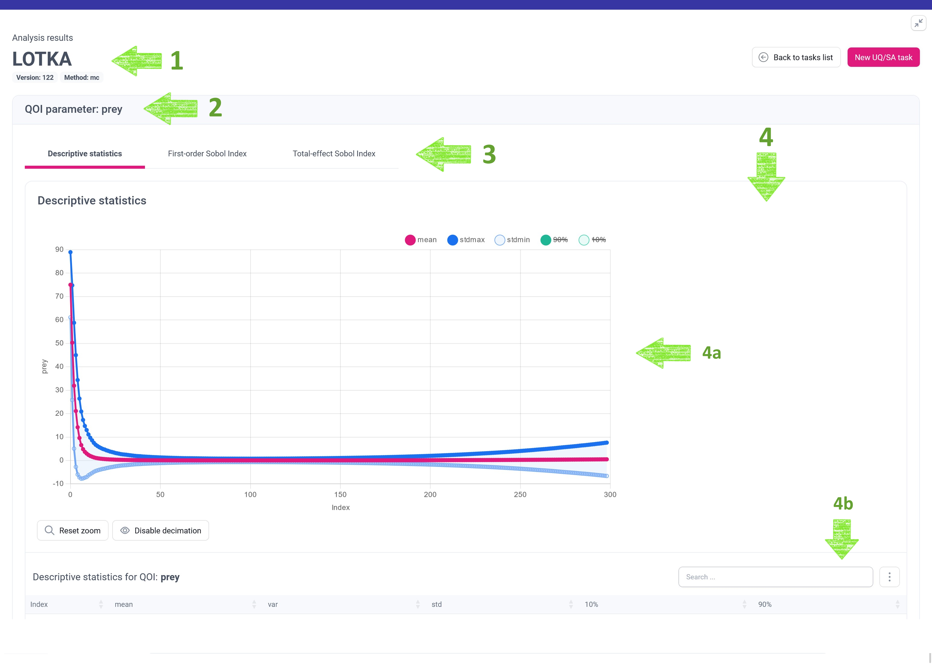
Let’s see what the green arrows indicate:
- High-level information about the analysis, including name of the analysis, version of the mUQSA template that has been used and the applied UQ/SA method.
- List of sections for one or many Quantities of Interests (QoIs). For the analysed case, there are two such sections, for prey and predator QoIs.
- Number of tab panes for different kinds of statistics generated by the selected mUQSA method for a given QoI.
- Panel presenting statistical data in a form adjusted to the selected statistic. Many panels include interactive charts (4a) and tables (4b).
The presentation of results by mUQSA also varies depending on the type of QoI: for the vector QoIs (models having a vector as an output) it is typically more extended than for the scalar QoIs (models having a scalar value as an output). The Lotka-Volterra model we are dealing with generates vector QoI, thus we can expect more elaborate presentation.
With this foundational knowledge in mind, we will now proceed to a brief presentation of the generated results for UQ/SA Lotka-Volterra. We will focus on the QoI for the prey, but the concept applies equally to the QoI for the predator.
Tip
For details on the mUQSA analysis function, see the documentation.
Descriptive statistics
The aim of Descriptive statistics is to provide general information about the uncertainty of the model. Consequently, the presented information includes the main statistical moments for the analysed QoI.
For the prey vector QoI, mUQSA uses two complementary methods for presenting descriptive statistics.
The first method entails a chart where the X-axis, labeled as Index, delineates the simulation’s time steps, while the Y-axis represents specific statistical moments like mean or standard deviation.
The second method involves a table where the rows correspond to the simulation’s time steps, and the columns depict various statistical moments. In addition, the table is equipped with a search field and the More button that offers both the ability to show or hide individual columns and to retrieve data stored in the table in different formats.
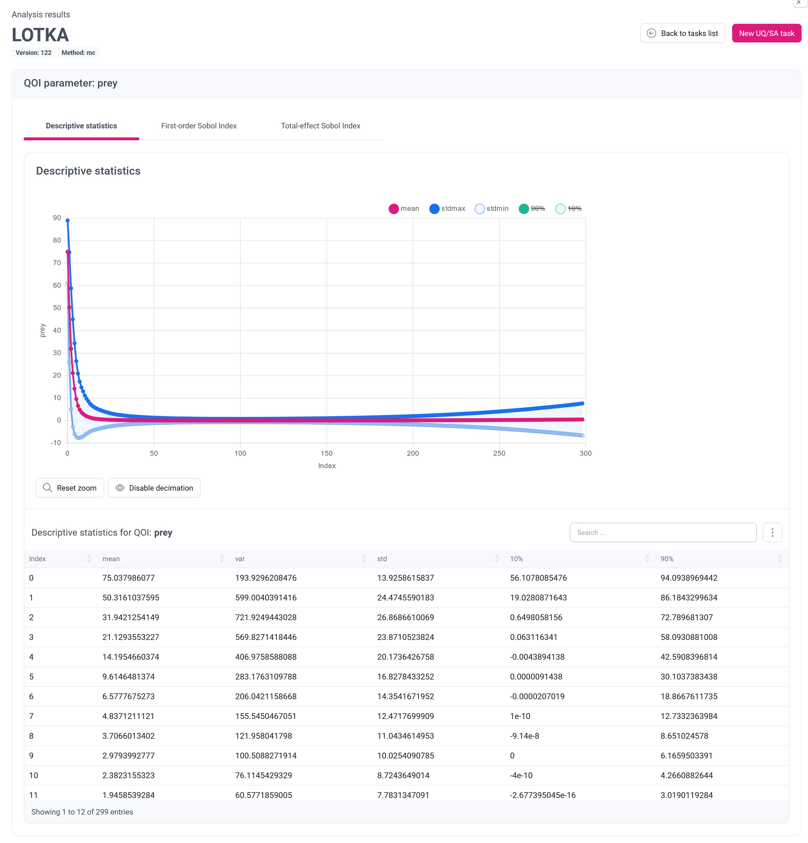
Analysing the data reveals certain patterns in the Quality of Interest (QoI). It exhibits a rapid decline, reaching a value below 1 after just 15 time-steps. However, higher-order moments indicate lingering uncertainty. Since this subtlety may not be immediately evident in the basic chart, mUQSA offers the capability to zoom in on the pertinent section of the data for closer examination.
Tip
To delve deeper into the most intriguing segment of the simulation, consider restricting the number of time-steps to around 50 while also boosting the number of method-generated samples. You may increase the MC method samples num, or explore alternative methods for further insight.
Sobol Indices
Sobol Index is a measure that allows to discover how the uncertainty of model parameters influences the output uncertainty. The result of Sobol’s analysis is a list of percentage values that displays a contribution of individual or combined input parameters variance on the variance of the results.
First-order Sobol Index displays the contribution of uncertainty of individual parameters on the output uncertainty. mUQSA presents this index in both graphical and tabular way. For the vector QoIs, the graphical presentation involves two-dimensional line chart, where the X-axis, labeled as Index, delineates the simulation’s time steps, while the Y-axis represents the value of Sobol Index for different input parameters.
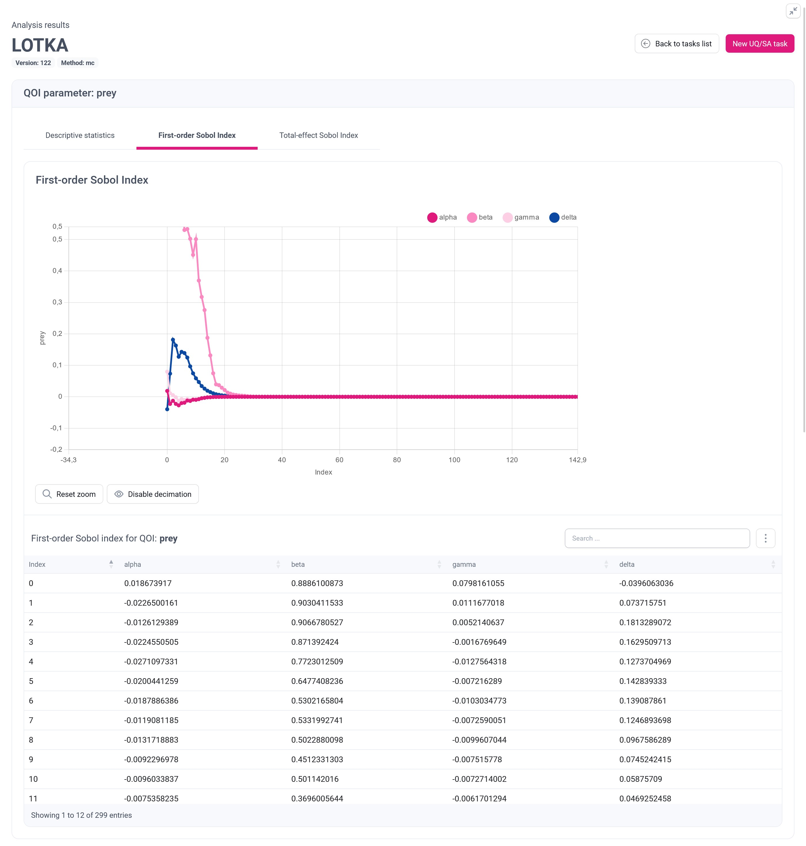
It becomes particularly apparent, especially when employing a zoomed view in the chart, that during the initial phase of the simulation, the $beta$ parameter has the most significant impact on the uncertainty of prey QoI, followed by the $delta$ parameter. After approximately 25 simulation steps, the uncertainty of input parameters becomes negligible for the output. This outcome is unsurprising, as by this point, the prey has likely been consumed by the predators.
Total-effect Sobol Index provides information about the complete contribution of input parameters uncertainty on the output uncertainty, including all interactions of a given parameter with other parameters. The presentation of Total-effect Sobol Index is analogous to the presentation of First-order Sobol Index.
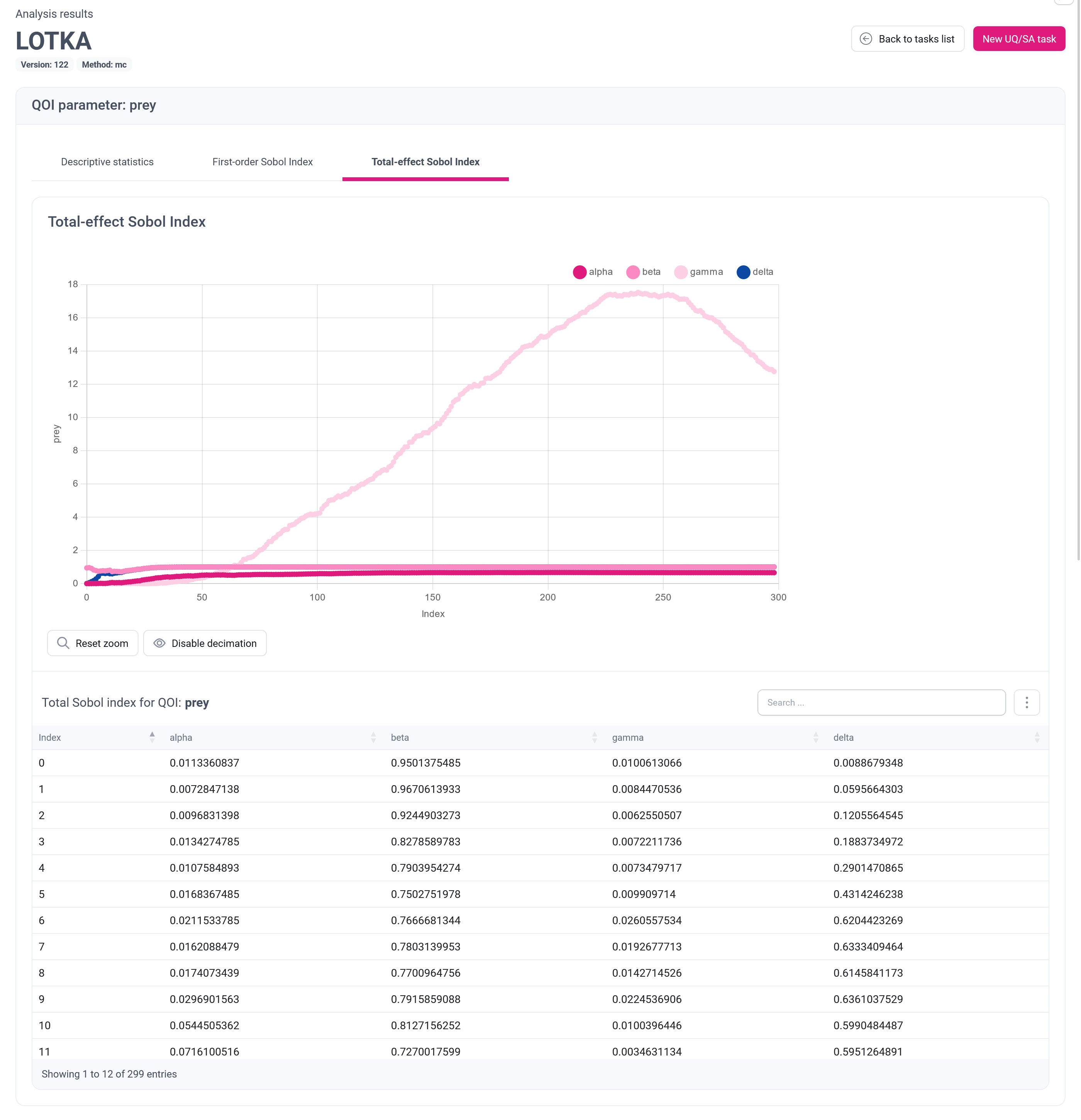
An intriguing observation in this example is the noteworthy increase in the value of the Total-effect Sobol Index for the parameter $gamma$. To elucidate this behavior, we need to revisit the descriptive statistics and the First-level Sobol Index. As you recall, the prey population diminishes rapidly, nearly reaching zero for the majority of the simulation. Consequently, while there may be a relative influence of $gamma$ and its interactions on the output, given that the output itself approaches zero, the practical impact is negligible. This rather intricate behavior underscores the true value of comprehensive, multifactorial analysis.
Acquiring raw data
In addition to graphical and tabular presentation of data, mUQSA gives users the option to access the generated data in raw format. This is especially important for advanced scenarios where further analysis in external software may be required.
The data can be accessed via embedded file explorer on the Results view, from which a user can display or download files.